Print Version - Center for the Biology of Natural Systems

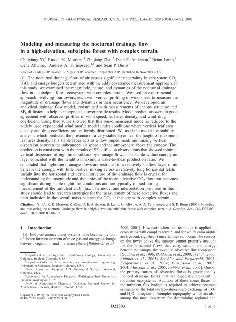
JOURNAL OF GEOPHYSICAL RESEARCH, VOL. 110, D22303, doi:10.1029/2005JD006282, 2005Modeling and measuring the nocturnal drainage flowin a high-elevation, subalpine forest with complex terrainChuixiang Yi, 1 Russell K. Monson, 1 Zhiqiang Zhai, 2 Dean E. Anderson, 3 Brian Lamb, 4Gene Allwine, 4 Andrew A. Turnipseed, 1,5 and Sean P. Burns 1Received 27 May 2005; revised 17 August 2005; accepted 1 September 2005; published 16 November 2005.[1] The nocturnal drainage flow of air causes significant uncertainty in ecosystem CO 2 ,H 2 O, and energy budgets determined with the eddy covariance measurement approach. Inthis study, we examined the magnitude, nature, and dynamics of the nocturnal drainageflow in a subalpine forest ecosystem with complex terrain. We used an experimentalapproach involving four towers, each with vertical profiling of wind speed to measure themagnitude of drainage flows and dynamics in their occurrence. We developed ananalytical drainage flow model, constrained with measurements of canopy structure andSF 6 diffusion, to help us interpret the tower profile results. Model predictions were in goodagreement with observed profiles of wind speed, leaf area density, and wind dragcoefficient. Using theory, we showed that this one-dimensional model is reduced to thewidely used exponential wind profile model under conditions where vertical leaf areadensity and drag coefficient are uniformly distributed. We used the model for stabilityanalysis, which predicted the presence of a very stable layer near the height of maximumleaf area density. This stable layer acts as a flow impediment, minimizing verticaldispersion between the subcanopy air space and the atmosphere above the canopy. Theprediction is consistent with the results of SF 6 diffusion observations that showed minimalvertical dispersion of nighttime, subcanopy drainage flows. The stable within-canopy airlayer coincided with the height of maximum wake-to-shear production ratio. Weconcluded that nighttime drainage flows are restricted to a relatively shallow layer of airbeneath the canopy, with little vertical mixing across a relatively long horizontal fetch.Insight into the horizontal and vertical structure of the drainage flow is crucial forunderstanding the magnitude and dynamics of the mean advective CO 2 flux that becomessignificant during stable nighttime conditions and are typically missed duringmeasurement of the turbulent CO 2 flux. The model and interpretation provided in thisstudy should lead to research strategies for the measurement of these advective fluxes andtheir inclusion in the overall mass balance for CO 2 at this site with complex terrain.Citation: Yi, C., R. K. Monson, Z. Zhai, D. E. Anderson, B. Lamb, G. Allwine, A. A. Turnipseed, and S. P. Burns (2005), Modelingand measuring the nocturnal drainage flow in a high-elevation, subalpine forest with complex terrain, J. Geophys. Res., 110, D22303,doi:10.1029/2005JD006282.1. Introduction[2] Eddy covariance tower systems have become the toolof choice for measurement of trace gas and energy exchangebetween vegetation and the atmosphere [Baldocchi et al.,1 Department of Ecology and Evolutionary Biology, University ofColorado, Boulder, Colorado, USA.2 Department of Civil, Environmental, and Architectural Engineering,University of Colorado, Boulder, Colorado, USA.3 Water Resources Discipline, U.S. Geological Survey, Lakewood,Colorado, USA.4 Laboratory for Atmospheric Research, Washington State University,Pullman, Washington, USA.5 Now at Atmospheric Chemistry Division, National Center forAtmospheric Research, Boulder, Colorado, USA.Copyright 2005 by the American Geophysical Union.0148-0227/05/2005JD006282$09.002000, 2001]. However, when this technique is applied toecosystems with complex terrain, and for which calm nightsare frequent, significant uncertainties can occur. The sensorson the tower above the canopy cannot properly accountfor the horizontal flows that carry scalars and energybeneath the canopy, the so-called advective flux component[Goulden et al., 1996; Baldocchi et al., 2000; Yi et al., 2000;Aubinet et al., 2003; Staebler and Fitzjarrald, 2004;Feigenwinter et al., 2004; Turnipseed et al., 2003,2004; Marcolla et al., 2005; Aubinet et al., 2005]. One ofthe primary causes of advective fluxes is gravitationallyinduced drainage flows that are especially prevalent inmountain ecosystems. Addition of these mean fluxes tothe turbulent flux budget is required to achieve accurateestimates of the total surface-atmosphere exchange of CO 2and H 2 O. In regions of complex topography, which are alsoamong the most important for determining regional andD223031of13

D22303YI ET AL.: DRAINAGE FLOW MODELD22303global carbon and water budgets [Barry, 1993; Schimel etal., 2002], the characterization of drainage flows and theirassociated advective fluxes is especially important.[3] One line of evidence for the occurrence of drainageflows is the within canopy, S-shaped, wind profile that hasbeen widely observed [Fons, 1940; Allen, 1968; Bergen,1971; Oliver, 1971; Landsberg and James, 1971; Shaw,1977; Lalic and Mihailovic, 2002; Turnipseed et al., 2003].The S-shaped profile refers to a second wind maximum thatis often observed within the trunk space of forests and aminimum wind speed in the region of greatest foliagedensity [Shaw, 1977]. The second wind maximum is likelydue to the combined effect of local drainage flows that canachieve relatively high speeds in the lower region ofthe canopy (D.E. Anderson et al., Mean advective fluxof CO 2 in a high elevation subalpine forest duringnocturnal conditions, submitted to Agricultural and ForestMeteorology, 2005, hereinafter referred to as Anderson etal., submitted manuscript, 2005), and resistance to the meanwind flow that can reduce wind speeds in the region of thecanopy with high leaf area density [Massman, 1997;Massman and Weil, 1999; Mohan and Tiwari, 2004; Poggiet al., 2004]. The factors that most determine the potentialfor drainage flows are terrain slope and nocturnal radiativecooling of the slope surface [Fleagle, 1950; Manins andSawford, 1979; Doran and Horst, 1981; Mahrt, 1982].Although past modeling efforts have replicated localdrainage flows across sloped terrain [Mahrt, 1982], to ourknowledge, no analytical mathematical model has yetpredicted the second wind maxima within the context ofthe entire vertical wind profile. It would be of great benefitto have such a model as its use would move us closer tobeing able to close scalar and energy budgets for bothmodeled and measured flux footprints. It would alsoprovide us with even better tools for modeling the processesof scalar and energy fluxes, and thus producing greateraccuracy in our predictions of the effects of environmentalchange on ecosystem biogeochemical cycles.[4] Our past observations of wind flow patterns at theNiwot Ridge Ameriflux site have revealed the presence ofthe secondary wind maximum, especially during nights withhigh atmospheric stability [Turnipseed et al., 2003]. Weinitially attributed the near-surface maximum as being dueto nighttime drainage flows. In a subsequent study, we usedan array of four towers, each with vertical profiling of CO 2and, at least, two-dimensional wind speed to estimate themagnitude and dynamics of horizontal mean advective CO 2fluxes (Anderson et al., submitted manuscript, 2005). In thecurrent study, we continued analysis of the drainage flowpatterns using the four-tower experimental design. Inorder to interpret our observations, we developed a onedimensionalanalytical model that is able to predict theS-shaped wind profile. We constrained the model withobservations of forest canopy structure, including detailedobservations on the vertical distribution of leaf area density,and we validated some of the model predictions using anSF 6 release experiment. Finally, we tested the analyticalmodel against a numerical model developed with computationalfluid dynamics (CFD) techniques; the latter modelrepresents a more detailed, mechanistic model. Overall, ouraim was to provide more insight into the dynamics andcauses of drainage flows in this ecosystem, and prepare ameans of ultimately assessing the effect of bias in the meanhorizontal and vertical flux components on the overall massbalance for CO 2 at the study site.2. Measurements2.1. Study Site[5] The studies were conducted at the Niwot Ridge Amerifluxsite located in a subalpine forest ecosystem in the RockyMountains of Colorado (40°1 0 58 00 N; 105°32 0 47 00 W, 3050 melevation), approximately 25 km west of Boulder and 8 kmeast of the Continental Divide. The terrain of the site has aslope of approximately 5°–7° within 400 m in the east-westdirection. Detailed maps showing the site topography havebeen presented in past papers [Turnipseed et al., 2003,2004]. Predominant winds are from the west [Brazeland Brazel, 1983], flowing downslope. Summertimemeteorology produces valley-mountain airflows, withthermal-induced, near-surface upslope winds from the eastoccurring on many afternoons. Nighttime flow is nearlyalways from the west, and is often katabatic (downslopedrainage). The surrounding subalpine forest is 100 yearsold, having recovered from clear-cut logging. Verylittle understory canopy is present due to the thin, oftendry soils at the site. Other details for the site can befound in Monson et al. [2002] and Turnipseed et al.[2002].2.2. Tower Profile and EddyCovariance Measurements[6] A multiple-tower observing system was employedwhich is capable of measuring eddy fluxes and verticalprofiles of the mixing ratios of CO 2 ,H 2 O, wind speed andwind direction. This system consists of four towers: ET(east tower); WT (west tower); NT (north tower) and ST(south tower) (Anderson et al., submitted manuscript,2005). The ET and WT towers are located 150 m apartand are oriented on a west-east (240°–60°) transect. TheNT and ST towers are 150 m apart along the 330°–150°transect. Thus the four towers form the vertices of adiamond, with the west-east points of the diamond alignedalong the westerly wind vector known to dominate nighttimeflows. Eddy covariance fluxes of CO 2 , water vapor andsensible heat were measured on the two west-to-east alignedtowers. The ET tower measurement height was 21.5 m andthe WT tower measurement height was 33 m. Verticalprofiles of scalar mixing ratios, wind speed and winddirection were measured at five levels on the ET and WTtowers (1, 3, 6, 10, and 21.5 m on ET tower; 1, 3, 6, 10, and33 m on WT tower), and at two levels on the two shortertowers (1, 6 m on NT and ST towers). Wind speedand direction were measured with at least two-dimensional,and at several heights three-dimensional, sonic anemometers.The instrumentation, calibration scheme and fluxcalculation methodology have been described in detailby Anderson et al. (submitted manuscript, 2005) andTurnipseed et al. [2002, 2003, 2004].2.3. Leaf Area Density Measurements[7] Canopy structure was studied in sixteen 10 10 mplots, eight directly east and eight directly west of the ETflux tower. The first plot was established at 50 m east or2of13

D22303YI ET AL.: DRAINAGE FLOW MODELD2230350 m west of the tower, with subsequent plots established at20 m intervals. Each tree greater than 1 m in height wasmeasured in all plots (total of 839 trees) for diameter atbreast height, height to crown and maximum diameter ofcrown (typically at the base of the crown) in the N-S andE-W perpendicular coordinates, and total tree height. Aseparate survey was done of 90 representative trees(30 lodgepole pines, 30 subalpine firs, and 30 Engelmannspruces) in the plots, evaluating diameter at breast heightagainst number of branches in the upper, middle and lowerthird of the trees, using binoculars to count branches. Wefound this approach to be accurate to within 10% whenchecked against a subset of ten trees accessible by canopyaccess towers at the site; the open nature of the forest, andthin nature of the tree crowns also facilitates accurateviewing with binoculars. Linear regression models predicted37–54%, 6–24%, and 1–30% of the variance inbranch number by diameter at breast height in the top,middle and bottom sections of the trees, respectively.Representative branches from the upper, middle and lowerthird of the crown in 30 trees equally distributed amongeach of the three dominant tree species were cut at theirintersection with the bole and measured for total needle drybiomass. Needle mass was converted to needle area using aregression constructed from separate analyses of sun andshade needles in 10 trees from each of the three species.Needle areas were determined with the water immersionmethod described by Chen et al. [1997]. From knowledgeof needle area per branch, branch number per unit bolediameter, average branch length in the top, middle andbottom thirds of the canopy, and total canopy height anddiameter (average diameter of the east-to-west and north-tosouthcrown diameter measurements), we estimated theaverage leaf area index (LAI) in 10 cm, concentric circlesfor each vertical third of the canopy for each of the 839 trees.We assumed that the vertical distribution of LAI in eachthird of the canopy decreased linearly from the bottom tothe top in 1 m thick layers. From these calculations, wewere able to estimate the leaf area density (leaf area per unitvolume) for each 1 m thick vertical layer of the crown ofeach tree. The leaf area density was summed for all trees ina plot for each vertical layer between the ground and 16 m(the maximum height of the canopy) and divided by thetotal area of the plot to provide a vertical profile of leaf areadensity for the entire plot.2.4. SF 6 Experiments[8] Sulfur hexafluoride (SF 6 ) tracer experiments wereconducted in July 2001 and 2002. In 2001, SF 6 was releasedcontinuously at a steady rate from a point source located at0.2 m above the forest floor approximately 50 m upslopefrom the WT tower. In 2002, SF 6 was released from a 200 mline source deployed across the slope at 0.2 m height and50 m upslope from the WT tower. Total release rates werecontrolled with a mass flow controller, and measurementsfrom the individual capillary restrictors (every 3 m along theline) were made from approximately 1/3 of the points duringeach test day. A fast response, continuous SF 6 analyzer wasoperated with the existing CO 2 ambient profiler system tomeasure SF 6 concentrations at 14 locations on the towers(ET, WT, ST, NT) in 2001 and 2002. The profiler sequentiallysamples for 30 s at each position and the measuredconcentrations are combined into 30 minute averages. Theanalyzer was calibrated using certified commercial standards(5% accuracy) during each test day. In this paper we onlyreport the results from a single SF 6 release during August2002; this was a period when all of the release anddetection instruments appeared to functioning at optimallevels, atmospheric stability was high, and the observeddrainage flows were strong.3. Theory[9] For simplicity, the atmosphere is assumed to bestable, incompressible and inviscid. Drainage flow is assumedto develop over a constant slope with angle a. Thecoordinate system used is Cartesian, with x in the directionof the mean downslope wind, and z normal to the slope. Thecanopy structure is assumed to be horizontally uniform butvaries in the vertical coordinate. No vertical motion andhorizontal static pressure gradient are considered, andCoriolis acceleration is neglected. For the steady statecondition, drainage flow is governed by [Wilson and Shaw,1977; Mahrt, 1982]:@u 0 w 0@zg Dq sin a ¼ c D ðÞ‘ z ðÞu z2 ðÞ; zq 0where u 0 w 0 is the average shear stress, g is theacceleration due to gravity, q 0 is the ambient potentialtemperature (in this case taken at 21.5 m height andthe influence of moisture on buoyancy is neglected), Dq =q q 0 is the deficit of potential temperature in thedrainage flow (where q is the potential temperature ofthe drainage flow), ‘(z) is the plant area density facingthe mean wind (defined as the frontal area of individualelements per unit volume of canopy), c D (z) =C D (z)/p(z)is the effective drag coefficient of plant elements subjectto a shelter factor p(z) within the canopy [Massman,1997; Massman and Weil, 1999], C D (z) is the foliage dragcoefficient, and u(z) is the average mean wind velocity.The drag coefficient within the canopy is definedaccording to Mahrt et al. [2000] asc D ðÞ¼ zu2 * ðÞ zu 2 ðÞ z:where u *(z) is the friction velocity within the canopy andis related to the shear stress asu 0 w 0 ¼ u 2 * ðÞ: zAfter substitution, equation (1) becomes@ ðc D ðÞu z2 ðÞ z Þ@zc D ðÞu z2 ðÞ‘ z ðÞ¼g zDq sin a:q 0The cumulative leaf area per unit ground area belowheight z is defined asZ zLz ðÞ¼0‘ ðz 0 Þdz 0 :ð1Þð2Þð3Þð4Þð5Þ3of13

D22303YI ET AL.: DRAINAGE FLOW MODELD22303Multiplying both sides of (4) by e L(z) and integratingfrom height z within the canopy to the top of the canopyh, we obtainu ðÞ¼ z eð LAI Lz ðÞÞc h Dc D ðÞ zu2 hgDq sin aq 0 c D ðÞ zZ hze!12ð Lz0 ð Þ Lz ðÞ Þ dz 0 ;ð6Þhwhere L(h) =LAI (the leaf area index), c D and u h arethe respective drag coefficient and mean wind speedat the top of the canopy. Equation (6), is to ourknowledge, the first analytical solution to the drainageflow problem inside a forest. Equation (6) retains the‘‘driving’’ force of gravity and ‘resistive’ force of canopyshear that govern the drainage flow and were originallyexpressed in equation (1). The solution in equation (6)covers the situations of downslope [u + (z)] and upslope[u (z)] wind speed. At our study site, the steady stateupslope flow [u (z)] is clearly restricted to daytimeperiods, and therefore will not be discussed further in thispaper. Hereafter, u(z) will refer solely to downslope windspeed [u + (z)], and in our consideration will be restricted tonighttime periods.[10] Prediction of the Reynolds stress, u 0 w 0 , profilewithin a canopy is important with regard to understandingthe complex interactions between wind flow and canopystructure [Shaw, 1977]. Several complicated higher-orderclosure models have been developed [e.g. Wilson and Shaw,1977; Katul and Albertson, 1998; Massman and Weil,1999]. A simple Reynolds stress model can be derivedusing our parameterization scheme. The drag force density,c D (z)u 2 (z), on the right hand side of equation (1) can bereplaced through equations (2) and (3) by the Reynoldsstress. Thus equation (1) becomes@u 0 w 0þ ‘ ðÞu z@z0 w 0 ¼ g Dq sin a:q 0When we repeat a similar procedure in the derivation ofequation (6), we obtain:u 0 w 0 ðÞ¼ zu 0 w 0 ðÞe hð LAI Lz ðÞÞg Dq sin aq 0Z hzeð7Þð Lz0 ð Þ Lz ðÞ Þ dz 0 ;where u 0 w 0 (h) is the Reynolds stress at the top of canopy. Ifthe terrain is flat, the dimensionless Reynolds stress profilebecomes:u 0 w 0 ðÞ zu 2 ðÞ h ¼ eð8Þð LAI Lz ðÞÞ; ð9Þwhere u 2 *(h) = u 0 w 0 (h). The relative Reynolds stress profileis determined uniquely by the function e (LAI L(z)) . We referto this function as a ‘canopy buffer function’ because itFigure 1. Dependence of slope-independent component ofcanopy wind profile on LAI predicted by equation (11)(with c D =0.11,c h D = 0.03, and u h = 2.93 m s 1 ).reflects the manner in which canopy structure influenceswind flow dynamics within the canopy.4. Results4.1. Application of the Model to a Forest CanopyWith Simple Structure[11] As an example of the model, we chose the simplecase in which the vegetation has a uniform vertical distributionof leaf area (‘(z) =‘ = cons.) and drag coefficient(c D (z)=c D = cons.). With these assumptions, equation (6) isreduced touz ðÞ¼where we usedch D u2 he LAI ð 1 hz Þ ghDq sin a1 e LAI 1 z 1ð hÞ2; ð10Þc D q 0 LAIc DR zLz ðÞLh ð Þ ¼ 0 ‘ ð z0 Þdz 0R h0 ‘ ð z0 Þdz ¼ z 0 h ; and ‘ ðÞ¼LAI z h :We can partition equation (10) into slope-independent andslope-dependent components. The slope-independent componentcan be written as:u fðÞ¼ zsffiffiffiffiffic h Dc Du h e LAI2 ð1 hz Þ : ð11ÞThis is the widely used exponential model for wind profilewithin a canopy [Inoue, 1963; Cionco, 1965; Cowan, 1968;Cionco, 1972; Raupach and Thom, 1981; Albini, 1981;Wilson et al., 1982; Massman, 1987; Macdonald,2000; Mohan and Tiwari, 2004]. The dependence of theslope-independent component on LAI is illustrated inFigure 1. The prediction from the model clearly reflectsthe overall influence of the canopy foliar density that resistsmean wind flow, and reduces wind speed to extremely lowvalues at high foliar densities. Using the same assumptions,the slope-dependent component can be written asu g ðÞ¼ zsffiffiffiffiffiffiffiffiffiffiffiffiffiffiffiffiffiffiffiffiffiffiffiffiffiffiffiffiffiffiffiffiffiffiffiffiffiffiffiffiffiffiffiffiffiffiffiffiffiffiffiffiffiffiffiffiffiffiffighDq sin a1 e LAI ð 1 hz Þ : ð12Þq 0 LAIc D4of13

D22303YI ET AL.: DRAINAGE FLOW MODELD22303Figure 2. Dependence of slope-dependent component ofcanopy wind profile on LAI predicted by equation (12) withtwo respective slopes: (a) a =5° and (b) a =15°. Thevalues of the rest of the parameters in equation (12) arespecified as c D =0.11,Dq = 2 K, and q 0 = 283 K.Equation (12) has a gravity-dependent driver that enhanceswind speed in the lower part of canopy, as shown inFigure 2. Foliar density impedes the gravitational flow,however, causing wind speed to decrease with increasing ofLAI, in the same manner as that for the slope-independentcomponent.[12] Under this uniform canopy structure condition, theReynolds stress profile (equation (8)) becomes:u 0 w 0 ðÞ¼ zu 0 w 0 hðÞe LAI 1ð hz Þ ghDq sin a1 e LAI ð 1 hz Þ :q 0 LAIð13ÞThe LAI dependence of the Reynolds stress is similar to thatof the mean wind speed as shown in Figures 1 and 2.4.2. Application of the Model to the NiwotRidge Canopy[13] We applied equation (6) to the Niwot Ridge forestcanopy to derive the vertical profile in canopy drag and topartition the influences of the slope-independent and slopedependentcomponents on the downslope drainage flowvelocity. In this derivation, we used the observed meanwind speed profile from two of the four towers (Figure 3).In using equation (6), the value for u h was taken from theanalysis shown in Figure 3 as 2.93 m s 1 ; values for u(z)were taken as the measured mean wind values at therespective heights reported in Figure 3. The upper part ofthe profile u(z) (i.e., above 10 m) was calculated by thesemilogarithmic wind profile:uz ðÞ¼ u *k ln z d : ð14Þusing von Karman’s constant (k) as 0.4 and u * as0.6 (m s 1 ). The displacement height (d) and roughnessz 0Figure 3. Averaged wind profile (circles) over nights (N =2556) in 2002. Points at level 1, 3, 6, 10, and 33 m weremeasured on the west tower (WT), the point at level 21.5 mwas measured on the east tower (ET). Data were onlyincluded that were available for all six levels within a singleaveraging period. Error bars for all points were smaller thanthe symbols. The line with horizontal dashes is a smoothedcurve. The upper part of the line was calculated by thesemilogarithmic wind profile as described by Turnipseed etal. [2003].length (z 0 ) under near-neutral atmospheric stability weretaken as 7.8 m and 1.16 m, respectively, which representmeasured values for the site [Turnipseed et al., 2003].Although the semilogarithmic law is probably invalid undermany conditions in the roughness sublayer [e.g., Raupachand Thom, 1981], it is the only tool we have available at thepresent time for smoothing the wind profile; it haslimitations in this analysis, which will be discussed shortly.[14] The drag coefficient profile was derived byequation (6) with, Dq = 2K,q 0 = 283 K, and slope a =5°(Figure 4). Mahrt et al. [2001] have shown that the surfaceFigure 4. The leaf area density profile (solid line)observed and drag coefficient profile (line with horizontaldashes) derived by equation (6). The circles and trianglewere the average drag coefficients calculated by equation (2)from the half-hour eddy covariance data at 1.5, 2.56, 5.7,and 21.5 m. The data used in the averages at 1.5, 2.56 and21.5 m occurred in the same averaging periods during thenights of 2002 (N = 1798), while the data used at 5.7 mwere in the nights of 2003 (N = 2603). The surface dragcoefficient observed at 21.5 m (triangle) is close to themodeled values at the top of canopy. The horizontal errorbars indicate ±1 standard error of the mean leaf area density.5of13

D22303YI ET AL.: DRAINAGE FLOW MODELD22303drag coefficient is independent of stability as wind speedexceeds 2 m s 1 for forests. The value c h D = 0.03 (for u h =2.93 m s 1 ) is close to the range of values observed byMahrt et al. [2001] in representative forests. Drag coefficients(circles and triangle in Figure 4) were obtained ina two-step calculation: half-hour values were first calculatedby equation (2) and then averaged for each level overthe entire nighttime period. The order of calculation willinfluence the estimated values due to the nonlinearity inequation (2). The records with small stress (u *< 0.01 m s 1and weak wind speeds

D22303YI ET AL.: DRAINAGE FLOW MODELD22303speed and air temperature (Figure 8). Using the Richardsonnumber (Ri) [Thom, 1971] defined asRi ¼g @Tq 0 @z@u@z 2!1Figure 6. Dimensionless Reynolds stress profile predictedby equation (8): triangles, total Reynolds stress; diamonds,slope-independent component; squares, slope-dependentcomponent; circles, observations. The observed data pointswere obtained from the same data sets as in Figure 4.Reynolds stress profile (Figure 7). Predictions of the stressprofile using our simple model were similar to those fromthe Wilson and Shaw (WS) model and in better agreementthan other past models.4.3. Prediction of a Very Stable Air Layer Withinthe Canopy[19] The vertical profile of wind speed predicted byequation (6) provides evidence of a layer with relativelylow flow between 3 and 6 m above the ground (Figure 3).This layer lies immediately below the layer of maximumleaf area density. We confirmed the existence of the stablelayer using measurements of the vertical profile in windwith @u/@z = 0 (Figure 8a) and @T/@z 6¼ 0 (Figure 8b), weobserved maximum stability at 6 m when the above-canopyatmosphere was stable (0.05 (z d)/L) and 3 m when theabove-canopy atmosphere was neutral ( 0.05 < (z d)/L

D22303YI ET AL.: DRAINAGE FLOW MODELD22303The shear production rate is usually expressed asP s ¼u 0 w 0 @u@z :ð19ÞThe ratio of the wake and shear production rates is thereforeP w¼ u @u0 w 0@zP s u 0 w 0 @u : ð20ÞSubstituting equations (2) and (3) into equation (20), theratio is reduced to@zP w¼u@c D=@zP s c D @u=@z þ 2 : ð21ÞFigure 9. Half-hour average of SF 6 concentrations at fourtowers during the period 0146–0504 LT on 8 August 2002.During the observation period we observed the typicalS-shaped wind profile (see Figure 10) and the meanObukhov stability was calculated as z =(z d)/L 5.87,indicating highly stable atmospheric conditions above thecanopy (at 21.5 m).optimal performance, we made observations of verticaldispersion at all four observation towers (Figure 9). Therewas clear sharp stratification among even the lowest observationlayers on the WT tower only 50 m downslope fromthe release line, indicating the presence of a thin downslopeflow with little upward mixing. By the time the tracer-ladenair reached the lower towers, there was evidence of somevertical mixing to the 6 m layer, but essentially none in thelayers above 8 m, even at the lowermost tower, 200 mdownslope from the release line. At the south tower (ST)and north tower (NT) we only made observations at thelowest vertical levels; however even at these levels, therewas sharp stratification between the lowest and highestlevels.4.4. Wake-to-Shear Production Rate as a PossibleCause of the Within-Canopy Stable Layer[21] We hypothesized that the stable, within-canopy layeris due to a localized region of high wake-to-shear productionratio. We explored this hypothesis using the analyticalmodel. Ignoring the slope-dependent term in equation (1)we can writeThus the ratio can be estimated on the basis of the windprofile presented in Figure 3 and the drag coefficient profilepresented in Figure 4. Qualitatively, the vertical gradient ofthe drag coefficient is almost opposite to that of wind speed.If the wake-to-shear production ratio is physically limited tobe positive, then it should be theoretically less than or equalto 2.[22] The ratio for the upper part of the canopy calculatedby equation (21) based on the wind and drag coefficientprofiles is shown in Figure 11. Calculated values wereindeed less than 2, except in the lowest part of the canopy,where equation (21) may not be valid because @u/@z 0.The maximum wake-to-shear production rate appears nearthe canopy height of maximum leaf density level rather thannear the top of canopy as has been shown in wind tunnelexperiments [Raupach et al., 1986]. The relative wakeproduction rate decreases linearly to zero from near themaximum leaf area density level to the top of canopy;following the decrease in leaf area density that occurs in theupper canopy layers of these conically shaped trees. Weinterpret this pattern as reflecting the fact that wake turbulenceis caused by the small-scale pressure gradient associatedwith canopy elements and hence depends on leaf areadensity.@u 0 w 0@z¼c D ðÞ‘ z ðÞu z2 ðÞ¼f z D :ð17ÞPhysically, the drag force (form drag) f D is a directconsequence of noncommutation of differentiation and areaaveraging over a horizontal plane that intersects numerousplants, producing the pressure force [Wilson and Shaw,1977; Raupach et al., 1986]. The wake turbulent productionrate is the work done by the flow against the form drag andcan be written asP w ¼ uf D ¼ u @u0 w 0: ð18Þ@zFigure 10. Half-hour average of wind speed at the WTtower during the same period as the SF 6 was observed inFigure 9.8of13

D22303YI ET AL.: DRAINAGE FLOW MODELD22303where U i and U j are the Reynolds-averaged velocitycomponents in x i and x j directions, P is the Reynoldsaveragedpressure, T is the Reynolds-averaged air temperature,n is the air molecular kinematic viscosity, n t is theturbulent ‘‘eddy’’ viscosity, G = n/Pr is the temperatureviscous diffusion coefficient, and G t = n t /Pr is the turbulentviscous diffusion coefficient, where Pr is the Prandtlnumber, and q source is the energy source in the fluid. Theterm g i h(T T 1 ) represents the buoyancy force on fluidflow, where g i is the gravity acceleration in i direction, h isthe thermal expansion coefficient of air, and T 1 is thereference temperature. F D in equation (24) stands for thedrag force (pressure drop) exerted by plant elements,F D ¼ 1 2 K ru 2 ;ð26ÞFigure 11. The ratio of the wake and shear productionrates calculated from equation (21) based on the windprofile in Figure 3 and drag coefficient profile in Figure 4.[23] In order to examine the effect of leaf area density onwake production, we applied equations (11) to (21) to thecase of a uniform vertical distribution of LAI, which causesequation (21) to becomeP w¼2h@c D=@zþ 2 : ð22ÞP s c D LAIThe prediction by equation (22) with the meanvalues derived from the drag coefficient profile in Figure 4(@c D /@(z/h) = 0.067 and c D = 0.11) is shown in Figure 12.Wake-to-shear production rate increases linearly withincreasing LAI for LAI < 2 m 2 m 2 , is progressively morelimited in its increase for LAI 2m 2 m 2 , and approachesan asymptote near 2 as LAI !1.4.5. Simulations With Computational Fluid Dynamics[24] To verify the experimental and analytical results, wefurther simulated airflow within and above the canopy usingcomputational fluid dynamics (CFD) techniques. CFD canpredict the spatial and temporal distributions of air pressure,velocity, temperature, humidity, and scalar concentration, aswell as turbulence if any, by numerically solving theconservation equations for fluid flows. The present CFDsimulation solves the two-dimensional steady state incompressibleReynolds-averaged Navier-Stokes equations offluid flow, which can be expressed in a Cartesian coordinatesystem [Patankar, 1980; Anderson et al., 1984] aswhere K r is the resistance coefficient, which can be relatedto the porosity by an empirical relationship given by Hoener[1965]K r ¼ 1 2 3 2 12bð27Þwhere b is the porosity that can be determined from the leafarea density and drag coefficient profiles by assuming thatthe drag force term in equation (26) is equal to that inequation (1).[25] The turbulent ‘‘eddy’’ viscosity n t can be determinedthrough various turbulence models. In this study we used arenormalized group k-e turbulence model [Yakhot et al.,1992], which generally has better accuracy and numericalstability than the ‘‘standard’’ k-e model [Launder andSpalding, 1974]. Equations (23)–(25) with the turbulencemodel are not mathematically closed until boundary conditionsare specified for the flow field. The boundaryconditions involved in this study include (1) inflow, upwindwind profile specified with the semilogarithmic law and T =7°C; (2) outflow, leeward and sky with fixed static pressureof 1 atm; (3) ground, nonslip condition with negative heatflux of 20 W m 2 ; (4) internal objects (plants) withresistance and heat, the resistance is specified according toequation (26) and the long-wave radiation from the plants isspecified to linearly decrease from 63 W m 2 at the top@U i@x i¼ 0;ð23ÞU j@U i@x j¼@P þ @ ðn þ n t Þ @U i@x i @x j @x jg i hðT T 1 Þ F D ; ð24Þ@TU j ¼ @ ðG þ G t Þ @T þ q source@x j @x k @x kð25ÞFigure 12. The dependence of the ratio of the wake andshear production rates on LAI. The curve is predicted byequation (22) for given @c D /@(z/h) = 0.06 (mean valuederived from the drag coefficient profile in Figure 4) andc D =0.11.9of13

D22303YI ET AL.: DRAINAGE FLOW MODELD22303Figure 13. (a) Domain and (b) simulated two-dimensional canopy flow by the renormalized group k-eturbulence model. The drag coefficient profile derived from the analytical model and the leaf area densityprofile in Figure 4 were used as inputs in the numerical model. In this simulation, slope a =5°,temperature deficit DT = 6°C, and details for the boundary conditions are described in the text. Theflow field shown in Figure 13b is a snapshot of simulated results taken near the middle of the domain.The different gray shading in the background in Figure 13b indicates the wind speed contours. The whitearrows represent wind vectors that indicate wind direction and magnitude of wind speed. The total heightof the domain in the simulation is 50 m. The dark arrow on right-hand side of Figure 13b shows themodeled canopy height. Note the minimum wind speed that is reached at the approximate height of themidcanopy layer of maximum LAI and the secondary maximum wind speed that is reached in the lowercanopy trunk space.layer of the canopy to zero at the middle of canopy (i.e., thestable situation specified by Siqueira and Katul [2002]).[26] The flow-governing equations (23)–(25) withboundary conditions are highly nonlinear and self-coupled,which renders them impossible for analytical solution formost real cases. Hence, using CFD, we solve the equationsby dividing the spatial continuum into a finite number ofdiscrete cells and discretizing the equations using the finitevolume method (FVM), thus converting them to a set ofnumerically solvable algebraic equations. An iterative procedureis then used to obtain the solution for each discretefield and equations. More detailed descriptions of CFD aregiven by Patankar [1980] and Anderson et al. [1984].[27] In the present study we used a validated CFDprogram [Concentration Heat and Momentum Ltd., 1999]to simulate the forest canopy flow. The simulation dividesthe flow field into 200 200 = 40,000 cells in x-z section,which represents one computational node per 4 m in thex coordinate, per 0.15 m in the z coordinate withinthe canopy volume (0–16 m height), and per 0.56 m inthe z coordinate above the canopy (17–28 m height). Thecomputing time for such a simulation is about 4 hours on aPIII-900 MHz desktop PC. Figure 13 illustrates the computationaldomain and the calculated velocity vectors andcontours within and above the canopy. The secondary windspeed maximum due to drainage flow near ground andminimum wind speed near the canopy level with maximumleaf area density are clear in the CFD-simulated results(Figure 13b). Caution should be taken in interpreting thesimulated velocity field in the upper part of the domain(30–50 m) as the possible influence of larger-scale airmotions like mountain waves [Durran, 1990; Turnipseedet al., 2004] were not considered in this simulation. Overall,the simulated wind profile within and above the canopy is inexcellent agreement with the observations and analyticalsolution described in previous sections, especially below10 m (Figure 14). Small differences between the resultsfrom the CFD model and observations above the 10 mheight probably result from use of the semilogarithmic lawto smooth the observational wind profile. This would be10 of 13

D22303YI ET AL.: DRAINAGE FLOW MODELD22303Figure 14. Comparison of the simulated wind profilesfrom the CFD model (solid line), the analytical solution(equation (6)) (line with horizontal dashes), and observations(circles).consistent with past studies that have shown the localflux-gradient relationship [Raupach and Thom, 1981] to beinadequate in the roughness sublayer.[28] Figure 15 shows the two-dimensional canopy flowsimulated by the CFD model with the assumption of auniform vertical distribution of LAI. The exponentialcanopy wind profile as shown in Figure 1, rather than theS-shaped wind profile, resulted from the uniform distributioncondition; this is the same result produced from theanalytical solution (see above). The results from the uniformdistribution condition also showed the disappearance of thevery stable within-canopy air layer. Thus, using this independentmodeling approach, we see the clear effect ofcanopy structure, and its tendency to cause surface drag,on the vertical distribution of the horizontal wind speed andthe production of the ‘‘super’’ stable layer within the canopy.5. Conclusions[29] The analytical, one-dimensional flow model derivedin this study represents a breakthrough in the modeling ofthe S-shaped canopy wind profile. The model retains thefundamental features of past drainage flow models based ondifferential equations, including (1) the fact that S shape isdetermined by the flow resistance properties of canopystructure, i.e., the drag area of plant elements and associateddrag coefficient, and (2) that the primary forcing variablesdetermining flow wind speed near the ground surface arepotential temperature deficit and slope angle. Using theanalytical model, however, we showed that as height abovethe ground increases, the shape of the wind profile isprogressively more determined by the canopy drag profile,than by the gravitational driving force profile. The onedimensionalmodel is reduced to the widely used exponentialwind profile model under conditions where vertical leafarea density and drag coefficient are uniformly distributed.[30] Our one-dimensional model successfully predictedthe familiar S-shaped canopy wind profile and the Reynoldsstress profile in the same manner as considerably morecomplicated higher-order closure models and, as in the othermodels, avoided reliance on eddy viscosity (K theory),which often fails in forest canopies. Our model recognizesthe drag force as an essential component in describinginteractions between plants and air flow, and we expressthe Reynolds stress by coupling it to the drag force densitywithout introducing phenomenological relations. This is animprovement over past higher-order closure models whichintroduce phenomenological ‘tuning’ to achieve final closurein the higher-order quantities.[31] Through two independent modeling approaches, theanalytical model and a discretized CFD model, we showedthat the heterogeneous vertical distribution of leaf areaindex produces a stable within-canopy layer of air. Thestable layer acts like a lid that minimizes the verticalexchange of mass and momentum below and above thelayer. The stable layer appears to be the result of maximumwake production in the region of maximum leaf areadensity that is characterized by small-scale turbulence andhigh dissipation rates [Raupach and Shaw, 1982]. Thepresence and influence of the stable layer is supported bySF 6 diffusion observations. The existence of a stablewithin-canopy layer leads us to conclude that horizontalmean advective fluxes are restricted to a relatively shallowlayer of air beneath the canopy, with little vertical mixingacross a relatively long horizontal fetch. Vertical meanadvective fluxes are minimal in the subcanopy air space,but originate near the top of the canopy and are significantabove the canopy. The vertical structure of these advectivefluxes appears to be highly determined by the verticalstructure in leaf area density, and its effects on the profileof the horizontal wind speed. With particular reference tothe vertical advective flux, our discovery of a very stablelayer of air within the canopy has important ramificationsFigure 15. The simulated two-dimensional canopy flow by the renormalized group k-e turbulencemodel under uniform vegetation condition (c D = 0.042 and ‘ =0.22m 2 m 3 ). All other specifications forthis simulation are the same as in Figure 13. The symbols are the same as in Figure 13b.11 of 13

D22303YI ET AL.: DRAINAGE FLOW MODELD22303for understanding certain causal relationships. In the past,we reported the existence of a positive bias to the verticalmean wind speed (w) in the vicinity of the ET tower at thesite [Turnipseed et al., 2003]. Our original hypothesis wasthat the accumulation of drainage flows at the site could beforcing the flow upward. With knowledge about thewithin-canopy super stable layer, it would appear thatsuch flows originate in the canopy layers above the regionof maximum foliar density, not close to the ground asoriginally hypothesized. This issue is clearly in need offurther investigation.[32] Acknowledgments. This work was financially supported by agrant from the South Central Section of the National Institute for GlobalEnvironmental Change (NIGEC) through the U.S. Department of Energy(BER Program) (cooperative agreement DE-FC03-90ER61010) andthrough funds from the U.S. Department of Energy Terrestrial CarbonProcesses Program (TCP) (grant DE-FG02-03ER63637). Any opinions,findings, and conclusions or recommendations expressed in this publicationare those of the authors and do not necessarily reflect the views of the DOE.We are grateful for valuable discussions with William J. Massman. Thefacilities of the University of Colorado Mountain Research Station (MRS)and the support of Bill Bowman (Director of the MRS) and Steve Seiboldare gratefully acknowledged. We are grateful for permission by the U.S.Forest Service to conduct the studies in the Roosevelt National Forest.ReferencesAlbini, F. A. A. (1981), Phenomenological model for wind speed and shearstress profiles in vegetation cover layers, J. Appl. Meteorol., 20, 1325–1335.Allen, L. H., Jr. (1968), Turbulence and wind speed spectra within aJapanese larch plantation, J. Appl. Meteorol., 7, 73–78.Anderson, D. A., J. C. Tannehill, and R. H. Pletcher (1984), ComputationalFluid Mechanics and Heat Transfer, 599 pp., Taylor and Francis,Philadelphia, Pa.Aubinet, M., B. Heinesch, and M. Yernaux (2003), Horizontal and verticalCO 2 advection in a sloping forest, Boundary Layer Meteorol., 108, 397–417.Aubinet, M., et al. (2005), Comparing CO 2 storage and advection conditionsat night at different CARBOEUROFLUX sites, Boundary LayerMeteorol., 116, 63–94.Baldocchi, D. D., J. J. Finnigan, K. W. Wilson, U. K. T. Paw, and E. Falge(2000), On measuring net ecosystem carbon exchange in complex terrainover tall vegetation, Boundary Layer Meteorol., 96, 257–291.Baldocchi, D. D., et al. (2001), Fluxnet: A new tool to study the temporaland spatial variability of ecosystem-scale carbon dioxide, water vapor,and energy flux densities, Bull. Am. Meteorol. Soc., 82, 2415–2434.Barry, R. G. (1993), Mountain Weather and Climate, 402 pp., Metheun,New York.Bergen, J. D. (1971), Vertical profiles of windspeed in a pine stand, For.Sci., 17, 314–321.Brazel, A., and P. Brazel (1983), Summer diurnal wind patterns at NiwotRidge, CO, Phys. Geogr., 4, 53–61.Cescatti, A., and B. Marcolla (2004), Drag coefficient and turbulence intensityin conifer canopies, Agric. For. Meteorol., 121, 197–206.Chen, J. M., P. M. Rich, S. T. Gower, J. M. Norman, and S. Plummer(1997), Leaf area index of boreal forests: Theory, techniques, and measurements,J. Geophys. Res., 102, 29,429–29,443.Cionco, R. M. (1965), A mathematical model for air flow in a vegetationcanopy, J. Appl. Meteorol., 4, 517–522.Cionco, R. M. (1972), A wind-profile index for canopy flow, BoundaryLayer Meteorol., 3, 255–263.Concentration Heat and Momentum Ltd. (1999), PHOENICS, version 3.1,London.Cowan, I. R. (1968), Mass, heat, and momentum exchange between standsof plants and their atmospheric environment, Q. J. R. Meteorol. Soc., 94,318–332.Doran, J. C., and T. W. Horst (1981), Velocity and temperature oscillationsin drainage winds, J. Appl. Meteorol., 20, 360–364.Durran, D. R. (1990), Mountain waves and downslope winds, in AtmosphericProcesses Over Complex Terrain, edited by B. Blumen,pp. 59–81, Am. Meteorol. Soc., Boston.Feigenwinter, C., C. Bernhofer, and R. Vogt (2004), The influence ofadvection on the short term CO 2 -budget in and above a forest canopy,Boundary Layer Meteorol., 113, 201–224.Fleagle, R. G. (1950), A theory of air drainage, J. Meteorol., 7, 227–232.Fons, W. L. (1940), Influence of forest cover on wind velocity, J. For., 38,481–486.Goulden, M. L., J. W. Munger, S. M. Fan, B. C. Daube, and S. C. Wofsy(1996), Measurements of carbon sequestration by long-term eddy covariance:Methods and a critical evaluation of accuracy, Global ChangeBiol., 2, 169–182.Hoener, S. F. (1965), Fluid Dynamic Drag: Practical Information on AerodynamicDrag and Hydrodynamic Resistance, S. F. Hoener, MidlandPark, N. J.Inoue, E. (1963), On the turbulent structure of air flow within crop canopies,J. Meteorol. Soc. Jpn., 41, 317–326.Katul, G. G., and J. D. Albertson (1998), An investigation of higher orderclosure models for a forested canopy, Boundary Layer Meteorol., 89,47–74.Lalic, B., and D. T. Mihailovic (2002), A new approach in parameterizationof momentum transport inside and above forest canopy under neutralconditions, in Integrated Assessment and Decision Support: Proceedingsof the 1st Biennial Meeting of the International Environmental Modellingand Software Society, vol. 2, edited by A. E. Rizzoli and A. J. Jakeman,pp. 139 – 154, Int. Environ. Modell. and Software Soc., Manno,Switzerland.Landsberg, J. J., and G. B. James (1971), Wind profiles in plant canopies:Studies on an analytical model, J. Appl. Ecol., 8, 729–741.Launder, B. E., and D. B. Spalding (1974), The numerical computation ofturbulent flows, Comput. Methods Appl. Mech. Eng., 3, 269–289.Macdonald, R. W. (2000), Modelling the mean velocity profile in the urbancanopy layer, Boundary Layer Meteorol., 97, 25–45.Mahrt, L. (1982), Momentum balance of gravity flows, J. Atmos. Sci., 39,2701–2711.Mahrt, L., X. Lee, A. Black, H. Neumann, and R. M. Staebler (2000),Nocturnal mixing in a forest subcanopy, Agric. For. Meteorol., 101,67–78.Mahrt, L., D. Vickers, J. Sun, N. O. Jensen, H. Jorgensen, E. Pardyjak, andH. Fernando (2001), Determination of the surface drag coefficient,Boundary Layer Meteorol., 99, 249–276.Manins, P. C., and B. L. Sawford (1979), A model of katabatic winds,J. Atmos. Sci., 105, 1011 – 1025.Marcolla, B., A. Cescatti, L. Montagnani, G. Manca, G. Kerschbaumer, andS. Minerbi (2005), Importance of advection in the atmospheric CO 2exchanges of an alpine forest, Agric. For. Meteorol., 130, 193–206.Massman, W. J. (1987), A comparative study of some mathematical modelsof the mean wind structure and aerodynamic drag of plant canopies,Boundary Layer Meteorol., 40, 179–197.Massman, W. J. (1997), An analytical one-dimensional model of momentumtransfer by vegetation of arbitrary structure, Boundary LayerMeteorol., 83, 407–421.Massman, W. J., and J. C. Weil (1999), An analytical one-dimensionalsecond-order closure model of turbulence statistics and the Lagrangiantime scale within and above plant canopies of arbitrary structure, BoundaryLayer Meteorol., 91, 81–107.Mohan, M., and M. K. Tiwari (2004), Study of momentum transfer within avegetation canopy, Proc. Indian Acad. Sci. Earth Planet. Sci., 113,67–72.Monson, R. K., A. A. Turnipseed, J. P. Sparks, P. C. Harley, L. E. Scott-Denton, K. L. Sparks, and T. E. Huxman (2002), Carbon sequestration ina high-elevation, subalpine forest, Global Change Biol., 8, 459–478.Oliver, H. R. (1971), Wind profiles in and above a forest canopy, Q. J. R.Meteorol. Soc., 97, 548–553.Patankar, S. V. (1980), Numerical Heat Transfer and Fluid Flow, 197 pp.,McGraw-Hill, New York.Poggi, D., A. Porporato, L. Ridolfi, J. D. Albertson, and G. G. Katul(2004), The effect of vegetation density on canopy sub-layer turbulence,Boundary Layer Meteorol., 111, 565–587.Raupach, M. R., and R. H. Shaw (1982), Averaging procedures forflow within vegetation canopies, Boundary Layer Meteorol., 22,79–90.Raupach, M. R., and P. G. Thom (1981), Turbulence in and above plantcanopies, Annu. Rev. Fluid Mech., 13, 97–129.Raupach, M. R., P. A. Coppin, and B. J. Legg (1986), Experiments onscalar dispersion within a plant canopy, part I: The turbulence structure,Boundary Layer Meteorol., 35, 21–52.Schimel, D. S., T. G. F. Kittel, S. Running, R. K. Monson, A. A.Turnipseed, and D. Anderson (2002), Carbon sequestration studiedin western US mountains, Eos Trans. AGU, 83, 445, 449.Shaw, R. H. (1977), Secondary wind speed maxima inside plant canopies,J. Appl. Meteorol., 16, 514–521.Shaw, R. H., R. H. Silversides, and G. W. Thurtell (1974), Measurements ofmean wind flow and three-dimensional turbulence intensity within amature corn canopy, Agric. Meteorol., 13, 417–425.12 of 13

D22303YI ET AL.: DRAINAGE FLOW MODELD22303Siqueira, M., and G. G. Katul (2002), Estimating heat sources and fluxes inthermally stratified canopy flows using higher-order closure models,Boundary Layer Meteorol., 103, 125–142.Staebler, R. M., and D. R. Fitzjarrald (2004), Observing subcanopy CO 2advection, Agric. For. Meteorol., 122, 139–156.Thom, A. S. (1971), Momentum absorption by vegetation, Q. J. R.Meteorol. Soc., 97, 414–428.Turnipseed, A. A., D. E. Anderson, P. Blanken, and R. K. Monson (2002),Energy balance above a high-elevation subalpine forest in complextopography, Agric. For. Meteorol., 110, 177–201.Turnipseed, A. A., D. E. Anderson, P. D. Blanken, W. M. Baugh, andR. K. Monson (2003), Airflows and turbulent flux measurements inmountainous terrain. Part 1. Canopy and local effects, Agric. For.Meteorol., 119, 1 – 21.Turnipseed, A. A., D. E. Anderson, S. Burns, P. D. Blanken, and R. K.Monson (2004), Airflows and turbulent flux measurements in mountainousterrain. Part 2. Mesoscale effects, Agric. For. Meteorol., 125, 187–205.Wilson, J. D., D. P. Ward, G. W. Thurtell, and G. E. Kidd (1982), Statisticsof atmospheric turbulence within and above a corn canopy, BoundaryLayer Meteorol., 24, 495–519.Wilson, N. R., and R. H. Shaw (1977), A higher order closure model forcanopy flow, J. Appl. Meteorol., 16, 1197–1205.Yakhot, V., S. A. Orzag, S. Thangam, T. B. Gatski, and C. G. Speziak(1992), Development of turbulence models for shear flows by a doubleexpansion technique, Phys. Fluids A, 4, 1510– 1520.Yi, C., K. J. Davis, P. S. Bakwin, B. W. Berger, and L. Marr (2000), Theinfluence of advection on measurements of the net ecosystem-atmosphereexchange of CO 2 from a very tall tower, J. Geophys. Res., 105, 9991–9999.G. Allwine and B. Lamb, Laboratory for Atmospheric Research,Washington State University, Pullman, WA 99164-2910, USA.D. E. Anderson, Water Resources Discipline, U.S. Geological Survey,Denver Federal Center, Lakewood, CO 80225, USA.S. P. Burns, R. K. Monson, and C. Yi, Department of Ecology andEvolutionary Biology, University of Colorado, Boulder, CO 80309-0334,USA. (yic@colorado.edu)A. A. Turnipseed, Atmospheric Chemistry Division, National Center forAtmospheric Research, Boulder, CO 80305, USA.Z. Zhai, Department of Civil, Environmental, and ArchitecturalEngineering, University of Colorado, Boulder, CO 80309-0428, USA.13 of 13