CHAM CS - WES - Part 2

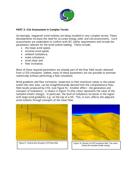
PART 2: Site Assessment in Complex TerrainIncreasingly, megawatt wind turbines are being installed in very complex terrain. Thesedevelopments increase the need for accurate energy yield- and site-assessments. Suchassessments are undertaken to confirm with IEC safety requirements and include theparameters relevant for the wind turbine loading. These include:• the mean wind speed,• extreme wind speed,• ambient turbulence,• wake turbulence,• wind shear and• flow inclination.Most of these required parameters are already part of the flow field results obtainedfrom a CFD simulation. Indeed, many of these parameters are not possible to estimaterealistically without performing a flow simulation.Wind gradients and flow inclination, respective to their maximum values or the valueswithin the rotor area, can be straightforwardly derived from the comprehensive flowfieldresults produced by CFD, (see Figure 9). Another effect - the generation andtransport of turbulence - is shown in Figure 10 (the colour represents the value of theturbulent kinetic energy). In particular, the level of turbulence increases in the regionwith large wind gradients; e.g. on the top of a hill. This, in turn, affects the adjacentwind turbines through transport of the mean flow.Figure 9: Vertical slice through a CFD flow-field.Figure 10: Section of CFD turbulence field. The colourshows the turbulent kinetic energy.

Figure 12 shows a colour map of thecharacteristic turbulence intensitydefined by the IEC standard. As theIEC proposes values of 18% and16% for the A and B classes, themap provides clear hints foroptimisation of the wind farm’sconfiguration.It should be noted that not allparameters are verified bymeasurements, because some of theparameters are difficult or evenimpossible to measure.2019181716151413However, it is already apparent thatstate-of-the-art flow simulation is thebest possible way to estimate these.Figure 12:Spatial variation of characteristicturbulence intensity calculated by CFD1210Hyperlink to primary textNote on elevation data processingIt is often asked how digital terrain data can be imported into PHOENICS. Inpractice, terrain data often comes in as height contour lines (e.g. DXF maps orWAsP map files), digitised from 1:25000 or 1:5000 topographical maps. Inorder to use that to construct a BFC grid with horizontal and vertical gridzooming, the contours must first be carefully interpolated to the defined surfacegrid nodes. Application of standard 2D-interpolation can lead to defects liketerrace forming between lines or overshoots. Therefore the "ray angleinterpolation" or one of its refinements may be used. For each grid point anumber of equally distributed "rays", and their intersection with the nearbycontours, are considered. An interpolation weight is assigned to each ray andits crossing contour, depending on the local angle between ray and contour,thus assigning higher weights to rays crossing a contour at 90° while assigninglower weights for sharper angles. The 3D BFC grid may be constructed on thisbasis over the surface and exported in ASCII grid format to PHOENICS, where itmay be smoothed using the Laplace grid smoothing tool. In order to promotenumerical properties, the initial surface may be slightly smoothed only in thevicinity of the outer grid boundaries. The level of detail of the initial heightmodel should fit to your horizontal grid spacing. In any case the resultingsurface grid needs to be inspected carefully.