2013 Lubbock Lecture - Phoenics

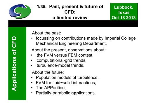
1/35. Past, present & future ofCFD:a limited reviewby Brian SpaldingLubbock,TexasOct 18 2013Applications of CFDAbout the past:• focussing on contributions made by Imperial CollegeMechanical Engineering Department.About the present, observations about:• the FVM versus FEM contest,• computational-grid trends,• turbulence-model trends.About the future:• Population models of turbulence,• FVM for fluid~solid interactions,• The APParition,• Partially-parabolic applications.

2/35. The Past:Before the digital ageLubbock,TexasOct 18 2013Airplanes appeared years before digital computers.Applications of CFDYet designers could even then predict their lift anddrag. They used a combination of potential-flowtheory with boundary-layer theory.This proceeded by iteration:1. First source-sink distributions were sought whichcaused streamlines to fit the airplane, which led to2. distributions of pressure over the surface.3.They then used boundary-layer theory to calculate the‘displacement thickness’ of the layer, i.e. the extent towhich the airplane seemed bigger than first assumed.4. Then they repeated steps 1, 2, 3; until convergence.

3/35. The Past: Is the pre-digitalmethod relevant today?Lubbock,TexasOct 18 2013Applications of CFDTheir boundary-layer theory was crude:• two-dimensional,• integral,• with assumed velocity profiles.Therefore wind-tunnel tests were needed in addition.But the principle was sound. And it still is;for computers remaintoo small to allowadequately fine ellipticgrids,despite the use ofmany levels ofsub-division.

4/35. The Past: CFD at IC MED;How we stumbled into itLubbock,TexasOct 18 2013Applications of CFDPrior to 1965, IC Mech Eng still used integral-profilemethods for 2D boundary-layer flows.Profiles were polynomials, with coefficients deducedfrom weighted-integral conservation equations.Then the Eureka-insight flash: piece-wise-linearprofiles were more flexible; with integration over‘pieces’; i.e. with unity weighting factors.We had invented (our own kind of) finite-volumeCFD.The rest is history.A remark aside: The finite-element community still usesnon-unity weighting factors; to their great disadvantage.One day they’ll learn. More about this later.

5/35. The Past at IC MED:Features of the first computerprogramLubbock,TexasOct 18 2013Applications of CFDIt first appeared in Patankar’s PhD Thesisof 1967, later published as a book.It simulated 2D parabolic flows, usingaxial distance and dimensionless streamfunction as co-ordinates, so minimisingfalse diffusion.The grid width expanded and contracted to cover onlythe region of interest. So it was ‘self-adaptive’.It handled turbulence via Prandtl’s mixing-length model.Wall functions made their first appearance in it.It used the TDMA, without iteration, for cross-streamsolution; and it ‘marched’ in the main-flow direction.

6/35. The Past at IC MED:More about 2D paraboliccomputer programsLubbock,TexasOct 18 2013Applications of CFDA second computer program, GENMIX, applied thesame method to more general 2D parabolic flows, e.g.wakes, plumes, wall jets for film-cooling, flames, etc.A major use was for systematic validation studies ofthe then-emerging two-equation turbulence models.It too was published as a book, with coding;and therefore used by non-IC researchers.However the IC group had already developedand published a stream-function~vorticityprogram for simulating 2D elliptic flows.We sought therefore a method to escape its restrictionsviz. to two dimensions; and to uniform density.

7/35. The Past at IC MED:SIVA, SIMPLE and 3DLubbock,TexasOct 18 2013Applications of CFDHarlow and Welch (1965) had published 3D methodsfor unsteady compressible flows; but our 2Dmethods handled practically more-important steadyand incompressible ones. We wanted to continue.Our first success was with SIVA (= SimultaneousVariable Adjustment) ( Caretto et al 1971). But itworked point-by-point and converged slowly.So SIMPLE came into existence, purloining elementsfrom predecessors, but surpassing them all (beinglater surpassed in its turn by SIMPLER, SIMPLEST,SIMPLEC, etc.)Later it was extended to two-phase, free-surface,magneto-hydrodynamics, and much more.

8/35. The Past at IC MED:3D parabolic and partially parabolicLubbock,TexasOct 18 2013Applications of CFDThe first publication of SIMPLE (1972) was for 3Dparabolic flows. This is fact seldom remembered.Eager to show SIMPLE’s elliptic capability, we tooquickly exemplified it. The world followed, and scarcelynoticed its parabolic capability. Who uses it nowadays?However, finding our computers too small (they still are;and may be forever), we later created the partiallyparabolicmethod. This stores 3D only pressures, butvelocities 2D, saving memory at the expense of time.There were numerous publication; but little world-widefollowing.Our fault, no doubt; but the world’s loss (I believe).More about this below.

9/35. The Past at IC MED:More about partially-parabolicLubbock,TexasOct 18 2013Applications of CFDIC’s publications concerned flows in curved and coiledtubes, rotating ducts, 2D turbines, and around ship’shulls. Too few! And with wrong emphasis.Their authors (I was one) compared partially-parabolicwith fully-parabolic (and therefore incorrect) solutions,rather than with more accurate fully-elliptic ones.Another distraction was: did the turbulence modelsused fit the experiments? Beside the point.What should have been stressed was:Replacing fully-elliptic by partially-parabolic,1. scarcely affected accuracy or computer time, but2. greatly reduced computer memory requirement.When authors forget the point, most readers will miss it.

13/35. A typical SSFT problem:blade in hot gas, cooled internallyLubbock,TexasOct 18 2013Applications of CFDHot gas flows outside an internallycooledblade-like solid.The un-structured grid which isused is shown below.The smallest cells are placed nearthe curved solid-fluid interfaces.The picture above shows thewhole calculation domain, withgas inlet on the left and outlet onthe right.Also visible is the central tube,which introduces the cooling air.The problem is illustrative, withidealised geometry.

16/35. Pressure distribution in gasLubbock,TexasOct 18 2013Applications of CFDPressurecontoursin theflowinggas.Red ishigh; blueis low.Pressure iscomputed bySIMPLE forgas only.

18/35. Summary of experiences withFVM applied to solid-stress problemsLubbock,TexasOct 18 2013Applications of CFDMany comparisons with both analytical and finite-elementsolutions have been made.They confirm that FVM for stress-in-solids problems is practicable,accurate and economical; it is at least as good as FEM.This is a fertile field for research, still almost explored.SIMPLE works well for both fluid flow and solid stress; but surelybetter SSFT-specific algorithms can be found.Other questions remaining to be answered concern:relative advantages of staggered and collocated structured grids;and of (various kinds of) unstructured grids.Extensions are also required to time-dependent phenomena:• to large (enough to influence the flow) displacements; and• to non-linear and plastic deformations.

19/35. Present trends:grids for arbitrary body shapeLubbock,TexasOct 18 2013Applications of CFDFirst used were body-fitted-coordinate grids whichwere topologically Cartesian, i.e. still ‘structured’; butsometimes hard to create.Therefore unstructured grids with tetrahedral cells(copied from FEM) were popular for many years.Polyhedral cells followed.These too present creation difficulties; and the currenttrend is back to Cartesian, albeit sub-divided as in justshownsolid-stress example.Then surface curvature may be allowed for by use ofthe ‘Immersed-Boundary Method’ (IBM).

20/35. Present trends:early IBM examplesLubbock,TexasOct 18 2013Applications of CFDThe PHOENICS IBM viz.PARSOL, simulates, on theright, flow through alouvred wall. It looksrealistic. But quantitativeaccuracy is improbable.The same is true of thefootball stadium on theleft.Plausibility is easy to get.Reliable accuracy - muchharder.

21/35. Present trends:SPARSOL (Structured PARSOL)Lubbock,TexasOct 18 2013Applications of CFDSome versions of the IBM perform poorly for solidswhich are thin compared with grid cells; carefulcalculation of the intersection locations is necessary.However realism can indeed be procured, withsufficient care (see below).

22/35. Present grid trends:Various storage locationsLubbock,TexasOct 18 2013Applications of CFD1. Staggered: pressures and scalars at cell centres;velocities on cell boundaries. This is the natural choice.2. Collocated: all variables at cell centres. Sometimes(unwisely?) preferred.3.Other: Xcell (various). Seldom used, but havingmerit.In grid on right, scalars , e.g.temperatures are stored attriangle centroids.So they are 4 times (8 in 3D)as numerous as pressuresand velocities.

23/35. Present grid trends:How Xcell reduces false diffusionLubbock,TexasOct 18 2013Applications of CFDBlue fluid flows in from left, red frombelow. Grid is Cartesian staggered.Interface is blurred, with diagonallydirectedflow, as seen on right.This is well known false diffusiondue to upwind differencing.Less well known is that upwinddifferencing with Xcell grid causes noblurring at all for flow angles at 0, 90or 45 degrees, as shown on right.False diffusion does exist at otherangles, but less than without Xcell.

24/35. Present grid trends:More-advanced XcellLubbock,TexasOct 18 2013Applications of CFDCartesian sub-divided gridscan also be ‘triangularised’: seeright.Not all cells need to be‘triangularised’; only those wherescalar gradients are large.In another version of Xcell, velocities are also storedat triangle centroids. This is ‘semi-collocated’ Xcell.Because pressures and velocities are not stored atthe same points, it is free from the ‘checker-boarding’ailment of conventionally collocated grids.What might be termed a ‘smart-grid’ technology isemerging which is ‘solution adaptive’.

25/35. Present: turbulence-modeltrends in terms ofhow many population membersLubbock,TexasOct 18 2013Applications of CFDVariables of popular turbulence models, e.g. k-e, LES,are local averages; implied population has 1 member.Eddy-break-up model for combustion (1971) is most-used2-member example. Population theory is not new.Only 2-(or more)-member-population models canrepresent chemical reaction, swirling-flows, and unmixing.The next three slides concern an un-mixingexperiment, first performed in 1978, which no 1-member (i.e. conventional) model has ever been ableto simulate.Will any one accept the challenge?

26/35. Turbulence trends:The Stafford experimentLubbock,TexasOct 18 2013Applications of CFDFill the lower half of a glass-sided vesselwith coloured salty water, and the tophalf with clear fresh water.Connect electrodes to a battery.The salty water heats more rapidly than thefresh. The consequent Rayleigh-Taylorinstability causes mixing.Soon the vessel appears to be filled withcoloured fluid.Quickly switch off the current; then the two fluids startto un-mix!In the end, the original sharp interface is restored.

27/35. Turbulence trends:Mixing followed by unmixing(Sapozhnikov and Mitiakov, 2010)Lubbock,TexasOct 18 2013Applications of CFD

28/35. Turbulence trends:A 2-member population modelcan do itLubbock,TexasOct 18 2013Applications of CFDEach member hasits own verticaldirectionvelocity.One is +ve theother –ve. Valuesare calculated fromNavier Stokes.At the start (on the left), the volume fraction is unity in thebottom half and zero in the top half.Later (in the middle) fragments of salty fluid rise, and even beginto concentrate at the upper surface.Later still (on the right), the heating has stopped; so the saltyfragments, lose heat to the fresh water and fall down to the bottomagain. Just as the video showed.Two-member models can simulate both mixing and un-mixing.

29/35. The future – perhaps.Models of turbulence will usemulti-member populationsLubbock,TexasOct 18 2013Applications of CFDOne-member models in effectrepresent temperature by one unityordinate at calculated abscissa. Theyknow nothing about PDFs.Multi-member models: 1. focus onseveral calculated ordinates atarbitrary abscissae. 2. simulate intermember-physics;3. calculate PDFs;4. solve more equations; 5. generatemuch more information.Computation is cheap: ignorance is expensive.So surely multi-member models must become the norm.

30/35. The future – perhapsUse one (FVM) code for both solidstressand fluid/heat-flow problems?Lubbock,TexasOct 18 2013Applications of CFDCommon sense says ‘Yes!’; for the world-wide cost ofFEM-for-solid-but-FVM-for-fluid is enormous;and all because FEM carriedneedless pre-computer baggage (theNUWFs) into the computer age:and others have been gulledinto using it.And why?The pictureanswers.

31/35. The future – perhapsWill general-purpose CFD codessurvive?Lubbock,TexasOct 18 2013Applications of CFDMy answer? Yes, but underground.Apps, aka SimScenes, apply CFD to special classes ofequipment, i.e. Simulation Scenarios, via app-specificmenus and buttons.App users may knowno more about CFDthan apple eatersabout arboriculture.Apps and apples canbe equally healthy ifthe tree-roots are wellnourishedApps will dominate.by the underlying CFD code.

32/35. The future – perhaps:Revival ot the partiallyparabolicmethod?Lubbock,TexasOct 18 2013Applications of CFDThe revived methodwould solve thesimple potential-flowelliptic equationoutside boundarylayer, wake and jet.Inside each of these it would solve 3D parabolicNavier-Stokes equations on as fine a grid as needed(easy because only 2D storage is required).Elliptic and parabolic solutions would alternate,exchanging domain-boundary information each time.Why should this not work? Is it perhaps already used?

33/35. The future – perhaps:Partially parabolic forautomobiles?Lubbock,TexasOct 18 2013Applications of CFDEarly (1988) PHOENICSneedlessly solved ellipticNavier-Stokes far fromthe vehicle surface wherethe flow is inviscid.Near much of surface theflow is 3D parabolic.But elliptic Navier-Stokesmust be used for the wake.And behind wheels andwing mirrors.

34/35. The future – perhaps:Implementation of partiallyparabolicfor automobilesLubbock,TexasOct 18 2013Applications of CFDWhat is needed, in order to implement such a hybridsolution procedure, is:• a CFD code with 2D and 3D, elliptic and paraboliccapabilities (Note that PHOENICS is an acronym forParabolic Hyperbolic Or Elliptic Numerical IntegrationCode Series; so it will do);• a flexible module for grid-to-grid transfer andinterpolation of solved-for variables(PHOENICS has an embryonic one); and• a user-friendly module for problem set-up and runcyclecontrol (coming soon).Nothing of significant difficulty is involved.

35/35. The future – perhaps:Terrestrial applications ofpartially-parabolicLubbock,TexasOct 18 2013Applications of CFDUrban-air-flow and windfarmsimulations have apredominant flow direction.Analysis can be parabolicover most of volume, withembedded elliptic subdomainsof recirculation.Grid fineness can be varied accordingto accuracy needs of each region.This and many other possibleextensions of the partially-parabolicmethod promises a highly profitablefuture. Let’s help bring that about.The End