Urban Wind Flows - Cham

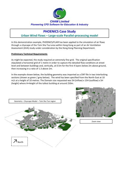
CHAM LimitedPioneering CFD Software for Education & IndustryPHOENICS Case StudyUrban Wind Flows – Large-scale Parallel-processing modelIn this demonstration example, PHOENICS/FLAIR has been applied to the simulation of air flowsthrough a cityscape of the Tsim Sha Tsui area within Hong Kong as part of an Air VentilationAssessment (AVA) study under consideration by the Hong Kong Planning Department.Preliminary Technical RequirementsAs might be expected, the study required an extremely fine grid. The original specificationstipulated a horizontal grid of 1 metre in order to capture the detailed flow conditions at streetlevel and between buildings and, vertically, at 0.5m for the first 4 layers below 2m above ground,then increasing in a ratio of 1.3 above 2m.In the example shown below, the building geometry was imported as a DXF file in two interlockingsections (shown as green / grey below). The wind has been specified from the North-East at 10m/s at a height of 10 metres. The Domain size requested was 5H (inflow) x 15H (outflow) x 5H(height) where H=Height of the tallest building at around 250m.Geometry - Cityscape Model – Tsim Sha Tsui regionZoom view↗North

Practical ConsiderationsThe CFD model described above involves a case size utilising ~100 million cells. Such a case is onlydeemed to be practical using 64-bit computer systems with a large RAM capacity, running inparallel-processing mode. Even then, the run times will be extremely lengthy involving daysrather than hours of CPU time.In view of the immediacy of the requirement stated by the customer, a reduced-size (yetrepresentative) case was created in preliminary form and is outlined below. The case was createdand performed on a Dell T7400 quad-core system with 16Gb RAM.Physical Domain size: 2587m * 1711m * 1000m (roughly 10H * 7H * 4H). In the X-Y plane, this isthe size of the geometry files supplied. The original specification is not precise enough to define adifferent domain size.Grid size: 744 * 704 * 45 (23.57 million cells). The grid was divided into 3 regions in X and Y. Thecentral region of 750m was assigned 500 cells, giving a cell-size of 1.5m. Outside the central zone,the grid was allowed to expand towards the domain boundaries. The largest cells at the domainboundaries were roughly 10m in size. In the Z (height) direction, the first 45m (up to the top ofthe green buildings) contained 17 uniform cells, the next 175m (up to the top of the highestbuilding) 15 cells expanding away from the ground and the remaining 778m to the sky boundary afurther 13 expanding cells.Wind Velocity: The wind speed at 10m was taken to be 10m/s, from the Northeast. A logarithmicprofile was used with a reference roughness height of 0.25m (equivalent to ‘scattered obstacles’).The geometry supplied had been exported from AutoCAD as a DXF file containing the surfaces ofthe roof tops. This file was used in AC3D to extrude down to the ground plane thus creating theclosed volumes required by PHOENICS. The resulting files were then imported into PHOENICS.Whilst PHOENICS has a variety of meshing options – Cartesian, Polar, Curvilinear and Unstructured– a Cartesian mesh was used. This is the most commonly mesh used for built environmentapplications of this type – ie a standard structured Cartesian mesh, coupled with the PARSOL cutcellfeature designed for handling complex geometries. PARSOL is described on CHAM’s web siteat: http://www.cham.co.uk/phoenics/d_polis/d_enc/in-form.htm.Similarly, the Chen-Kim k-epsilon model was selected from the many available within PHOENICS,as the most suitable for cases of this type.The inbuilt wind-profiling feature of PHOENICS/FLAIR was used. The wind speed is calculatedfrom:U/U * = ln(z/z o )/and the turbulence quantities are set to:k = U* 2 /0.3;= U* 3 /( *z)

where U is the total velocity at a height z from the ground; is von Karman's constant (=0.41), z ois the effective roughness height of the ground terrain; and U r is the reference velocity at thereference height z r . The total friction velocity U* is given by:U*= U r /ln(z r /z o )The reference velocity was taken to be 10m/s at a reference height of 10m. The effectiveroughness height was taken to be 0.25m.In this case, a WIND object was employed. As the wind direction does not match the grid, theWIND object decomposes the wind speed into the velocity components at the up-wind domainfaces and fixed pressure boundaries at the down-wind faces and the sky boundary. The WINDfeature allows changes in wind direction to be introduced easily.Treatment of terrainA terrain data file was supplied, but it did not appear to cover the same area as the geometryfiles. When it was imported at its nominal position, it covered a smaller area than the buildings,leaving a step on the ground plane. Many buildings also disappeared under the ground planewhich did not appear correct. The Tsim Shah Tsui area is predominantly flat in any case, hence, inthe interests of expedience, it was decided to omit the terrain object from the demonstration anduse a flat ground plane with a roughness height of 0.25m. In principle, any terrain would beimported and handled in the same manner as the buildings.ConclusionsOnce the initial geometry issues had been and established and resolved, the above reduced-sizecase was created and run with a few hours of man-time effort, and 72 hours of computer timewhen running in parallel-mode on a quad-core computer. The case occupied 13GB of RAM.The results readily show the variation in wind speed through the street canyons, areas of highturbulence, and calm regions. The plots shown below have been generated using the standardVR-Viewer post-processor which can display vectors, contours, iso-surfaces, high & low spots, andanimated view options.In the same way that alternative CAD products can be used for geometry creation and import intoPHOENICS, users also have the option to export the results to third-party post-processors [such asFEMView, Fieldview, Paraview, TECPLOT and Wavefront] for which interfaces are available withinPHOENICS.The case has been passed onto the customer for onward modification and refinement uponlarger-capacity computers to meet the stated meshing requirement. It should be noted that thedomain may need to be enlarged to meet the original specification, and the meshing increased toprovide the stated mesh density requirement. From a practical viewpoint, the resultingcalculation will be enormous, and it is then doubtful if it will produce substantially moremeaningful results, overall, than the reduced-size model. A more pragmatic solution would be toconcentrate mesh in particular areas of interest, rather than model the entire cityscape with thesame degree of accuracy.

ResultsThe following images were generated and are shown below:PLAN VIEW1. Wind velocity contours @ 2m above ground2. Wind velocity contours @ 5m above ground3. Wind velocity contours @ 10m above ground4. Wind velocity contours @ 20m above ground5. Wind velocity vectors @ 2m above ground6. Wind velocity vectors @ 5m above ground7. Wind velocity vectors @ 10m above ground8. Wind velocity vectors @ 20m above ground9. Zoom image - Wind velocity vectors @ 2m above ground10. Zoom image - Wind velocity vectors @ 5m above ground11. Zoom image - Wind velocity vectors @ 10m above ground12. Zoom image - Wind velocity vectors @ 50m above ground13. Zoom image - Wind velocity vectors @ 75m above ground14. Wind velocity contours @ 75m above ground15. Wind velocity vectors @ 75m above groundANGLED VIEW16. Zoom image - Wind velocity vectors @ 75m above ground17. Streamlines @ 2m above ground18. Streamlines @ 20m above ground19. Streamlines @ 50m above ground

↑North1. Wind velocity contours @ 2m above ground↙Wind2. Wind velocity contours @ 5m above ground

↑North3. Wind velocity contours @ 10m above ground↙ Wind4. Wind velocity contours @ 20m above ground

↑North5. Wind velocity vectors @ 2m above ground↙ Wind6. Wind velocity vectors @ 5m above ground

↑North7. Wind velocity vectors @ 10m above ground↙ Wind8. Wind velocity vectors @ 20m above ground

↑North9. Zoom image - Wind velocity vectors @ 2m above ground↙Wind10. Zoom image - Wind velocity vectors @ 5m above ground

↑North11. Zoom image - Wind velocity vectors @ 10m above ground↙ Wind12. Zoom image - Wind velocity vectors @ 50m above ground

A13. Zoom image - Wind velocity vectors @ 75m above ground↑North↙WindThe vector fields show interesting zones where the air direction is quite different from theprevailing wind. In Figures 9, 10 and 11 for example, the air near the building at the bottom left(labelled A in Fig 13) is travelling North. By 75m above ground, it is travelling South West and hasreversed direction. When the image is enlarged, similar features can be seen in many otherplaces. However, it can sometimes be hard to find individual regions of interest if the modelbecomes too cluttered by detail.

↗North14. Wind velocity contours @ 75m above ground←Wind15. Wind velocity vectors @ 75m above ground

16. Zoom image - Wind velocity vectors @ 75m above ground↗North←WindThe wakes behind the tall buildings can clearly be seen as blue zones of low velocity downstream,and as regions of higher velocity to the side.

↓North17. Streamlines starting @ 2m above ground↗WindThe streamlines are tracks of ‘mass-less’ particles. 150 tracks are started along the North face ofthe domain, and 100 along the East face. Here flow can be seen travelling up the street roughlyhalf-way along the domain. The buildings on either side are quite high and they protect the nearfloorflow from the prevailing wind. After a distance, the buildings on the right (West) sidebecome lower with an open space behind them. This allows the wind to pull the air out of thestreet canyon.The big green building on the left is forcing the air at this level to pass either side of it.The time shown on the scale is the time for the slowest track to reach the other side of thedomain. [The tracks start roughly 10m inboard of the domain edge, hence the short negativetime shown, which is the time the tracks took to reach the start line from the domain edge.]

↓North18. Streamlines starting @ 20m above ground↗ WindAt this height, the canyon effect is much less pronounced. The air now passes over the building onthe left. The group of tall buildings on the right act as a barrier forcing air sideways.

↓North19. Streamlines starting @ 50m above ground↗ WindAir is now mainly deflected upwards by the buildings below, with only the taller buildings acting asbarriers.CHAM Ltd, Bakery House, 40 High Street, Wimbledon Village, London SW19 5AU, UKTel: +44 (0)20 8947 7651 Fax: +44 (0)20 8879 3497 Email: phoenics@cham.co.ukWeb: http://www.cham.co.uk