Print Version - Center for the Biology of Natural Systems

More documents

Recommendations

Info

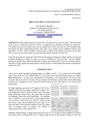
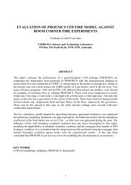
D22303YI ET AL.: DRAINAGE FLOW MODELD22303Figure 13. (a) Domain and (b) simulated two-dimensional canopy flow by the renormalized group k-eturbulence model. The drag coefficient profile derived from the analytical model and the leaf area densityprofile in Figure 4 were used as inputs in the numerical model. In this simulation, slope a =5°,temperature deficit DT = 6°C, and details for the boundary conditions are described in the text. Theflow field shown in Figure 13b is a snapshot of simulated results taken near the middle of the domain.The different gray shading in the background in Figure 13b indicates the wind speed contours. The whitearrows represent wind vectors that indicate wind direction and magnitude of wind speed. The total heightof the domain in the simulation is 50 m. The dark arrow on right-hand side of Figure 13b shows themodeled canopy height. Note the minimum wind speed that is reached at the approximate height of themidcanopy layer of maximum LAI and the secondary maximum wind speed that is reached in the lowercanopy trunk space.layer of the canopy to zero at the middle of canopy (i.e., thestable situation specified by Siqueira and Katul [2002]).[26] The flow-governing equations (23)–(25) withboundary conditions are highly nonlinear and self-coupled,which renders them impossible for analytical solution formost real cases. Hence, using CFD, we solve the equationsby dividing the spatial continuum into a finite number ofdiscrete cells and discretizing the equations using the finitevolume method (FVM), thus converting them to a set ofnumerically solvable algebraic equations. An iterative procedureis then used to obtain the solution for each discretefield and equations. More detailed descriptions of CFD aregiven by Patankar [1980] and Anderson et al. [1984].[27] In the present study we used a validated CFDprogram [Concentration Heat and Momentum Ltd., 1999]to simulate the forest canopy flow. The simulation dividesthe flow field into 200 200 = 40,000 cells in x-z section,which represents one computational node per 4 m in thex coordinate, per 0.15 m in the z coordinate withinthe canopy volume (0–16 m height), and per 0.56 m inthe z coordinate above the canopy (17–28 m height). Thecomputing time for such a simulation is about 4 hours on aPIII-900 MHz desktop PC. Figure 13 illustrates the computationaldomain and the calculated velocity vectors andcontours within and above the canopy. The secondary windspeed maximum due to drainage flow near ground andminimum wind speed near the canopy level with maximumleaf area density are clear in the CFD-simulated results(Figure 13b). Caution should be taken in interpreting thesimulated velocity field in the upper part of the domain(30–50 m) as the possible influence of larger-scale airmotions like mountain waves [Durran, 1990; Turnipseedet al., 2004] were not considered in this simulation. Overall,the simulated wind profile within and above the canopy is inexcellent agreement with the observations and analyticalsolution described in previous sections, especially below10 m (Figure 14). Small differences between the resultsfrom the CFD model and observations above the 10 mheight probably result from use of the semilogarithmic lawto smooth the observational wind profile. This would be10 of 13
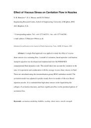
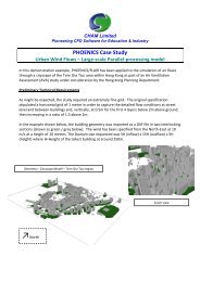
D22303YI ET AL.: DRAINAGE FLOW MODELD22303Figure 14. Comparison of the simulated wind profilesfrom the CFD model (solid line), the analytical solution(equation (6)) (line with horizontal dashes), and observations(circles).consistent with past studies that have shown the localflux-gradient relationship [Raupach and Thom, 1981] to beinadequate in the roughness sublayer.[28] Figure 15 shows the two-dimensional canopy flowsimulated by the CFD model with the assumption of auniform vertical distribution of LAI. The exponentialcanopy wind profile as shown in Figure 1, rather than theS-shaped wind profile, resulted from the uniform distributioncondition; this is the same result produced from theanalytical solution (see above). The results from the uniformdistribution condition also showed the disappearance of thevery stable within-canopy air layer. Thus, using this independentmodeling approach, we see the clear effect ofcanopy structure, and its tendency to cause surface drag,on the vertical distribution of the horizontal wind speed andthe production of the ‘‘super’’ stable layer within the canopy.5. Conclusions[29] The analytical, one-dimensional flow model derivedin this study represents a breakthrough in the modeling ofthe S-shaped canopy wind profile. The model retains thefundamental features of past drainage flow models based ondifferential equations, including (1) the fact that S shape isdetermined by the flow resistance properties of canopystructure, i.e., the drag area of plant elements and associateddrag coefficient, and (2) that the primary forcing variablesdetermining flow wind speed near the ground surface arepotential temperature deficit and slope angle. Using theanalytical model, however, we showed that as height abovethe ground increases, the shape of the wind profile isprogressively more determined by the canopy drag profile,than by the gravitational driving force profile. The onedimensionalmodel is reduced to the widely used exponentialwind profile model under conditions where vertical leafarea density and drag coefficient are uniformly distributed.[30] Our one-dimensional model successfully predictedthe familiar S-shaped canopy wind profile and the Reynoldsstress profile in the same manner as considerably morecomplicated higher-order closure models and, as in the othermodels, avoided reliance on eddy viscosity (K theory),which often fails in forest canopies. Our model recognizesthe drag force as an essential component in describinginteractions between plants and air flow, and we expressthe Reynolds stress by coupling it to the drag force densitywithout introducing phenomenological relations. This is animprovement over past higher-order closure models whichintroduce phenomenological ‘tuning’ to achieve final closurein the higher-order quantities.[31] Through two independent modeling approaches, theanalytical model and a discretized CFD model, we showedthat the heterogeneous vertical distribution of leaf areaindex produces a stable within-canopy layer of air. Thestable layer acts like a lid that minimizes the verticalexchange of mass and momentum below and above thelayer. The stable layer appears to be the result of maximumwake production in the region of maximum leaf areadensity that is characterized by small-scale turbulence andhigh dissipation rates [Raupach and Shaw, 1982]. Thepresence and influence of the stable layer is supported bySF 6 diffusion observations. The existence of a stablewithin-canopy layer leads us to conclude that horizontalmean advective fluxes are restricted to a relatively shallowlayer of air beneath the canopy, with little vertical mixingacross a relatively long horizontal fetch. Vertical meanadvective fluxes are minimal in the subcanopy air space,but originate near the top of the canopy and are significantabove the canopy. The vertical structure of these advectivefluxes appears to be highly determined by the verticalstructure in leaf area density, and its effects on the profileof the horizontal wind speed. With particular reference tothe vertical advective flux, our discovery of a very stablelayer of air within the canopy has important ramificationsFigure 15. The simulated two-dimensional canopy flow by the renormalized group k-e turbulencemodel under uniform vegetation condition (c D = 0.042 and ‘ =0.22m 2 m 3 ). All other specifications forthis simulation are the same as in Figure 13. The symbols are the same as in Figure 13b.11 of 13
Page 1 and 2: JOURNAL OF GEOPHYSICAL RESEARCH, VO
Page 3 and 4: D22303YI ET AL.: DRAINAGE FLOW MODE
Page 9: D22303YI ET AL.: DRAINAGE FLOW MODE
Page 13: D22303YI ET AL.: DRAINAGE FLOW MODE

Print Version - Center for the Biology of Natural Systems

You also want an ePaper? Increase the reach of your titles

Delete template?

Save as template?