Combined Reformulation of Bilevel Programming Problems

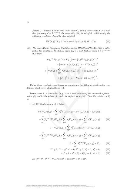
76(where C ◦ denotes a polar cone to the cone C) and if there exists K > 0 suchthat for every d ∈ R n+m+p the inequality (26) is satisfied. Additionally thefollowing condition should be also satisfied:∇F(¯x,ȳ) ⊤ d ≥ 0 ∀d ∈ conv T B ((¯x,ȳ,¯λ),H −1 (Γ)). (27)(iii) The weak Abadie Constraint Qualification for MPEC (MPEC-WACQ) is satisfiedat the point (¯x,ȳ,¯λ), if there exists K 1 > 0 such that for every d ∈ R n+m+pit follows:0 ≤ ∇F(¯x,ȳ) ⊤ d+K 1(‖max{0,(∇G IG (¯x,ȳ))d}‖ 2+ ∥ { max 0,(∇f(¯x,ȳ)) ⊤ d−V ↑ (¯x;d x ) }∥ ∥ 2p∑2+∥ ∇(∇ yf + λ i ∇ y g i )(¯x,ȳ,¯λ)d+‖∇g α (¯x,ȳ)d‖ 2∥i=1+ ∥ ∥∥d λγ 2+(ρC (−∇g β (¯x,ȳ)d,d λβ )) 2) 1 2.Under these regularity conditions we can obtain the following stationarity conditions,which were adapted from [13].Definition 3. Assume that (x,y,λ) is a local solution of the combined reformulation(5) and let the sets α, β, and γ be defined as in (15). Then the point (x,y,λ)is:1. MPEC M-stationary, if it holds:0 ∈ ∇ x F(x,y)+++m∑i=1m∑i=1k∑λ G i ∇ xG i (x,y)+λ V (∇ x f(x,y)−∂ ⋄ V(x))i=1λ KKTi ∇ x (∇ yi f +p∑λ j ∇ yi g j )(x,y)+j=10 = ∇ y F(x,y)+λ KKTi ∇ y (∇ yi f +p∑λ g i ∇ xg i (x,y) (28)i=1k∑λ G i ∇ y G i (x,y)+λ V ∇ y f(x,y)i=1p∑λ j ∇ yi g j )(x,y)+j=10 =m∑i=1p∑λ g i ∇ yg i (x,y)i=1λ KKTi ∇ yi g(x,y)−λ λ , (29)λ G ≥ 0, G(x,y) ⊤ λ G = 0, λ V ≥ 0, λ g γ = 0, λλ α = 0, (30)(λ g i > 0∧λλ i > 0)∨λ g i λλ i = 0, ∀i ∈ β, (31)for (λ G ,λ V ,λ KKT ,λ g ,λ λ ) ∈ R k ×R×R m ×R p ×R p .Publikacja objęta jest prawem autorskim. Wszelkie prawa zastrzeżone. Kopiowanie i rozpowszechnianie zabronione.Publikacja przeznaczona jedynie dla klientów indywidualnych. Zakaz rozpowszechniania i udostępniania w serwisach bibliotecznych