On the selection of primal unknowns for a FETI-DP formulation of the ...
On the selection of primal unknowns for a FETI-DP formulation of the ...
On the selection of primal unknowns for a FETI-DP formulation of the ...
- No tags were found...

You also want an ePaper? Increase the reach of your titles
YUMPU automatically turns print PDFs into web optimized ePapers that Google loves.
<strong>On</strong> <strong>the</strong> <strong>selection</strong> <strong>of</strong> <strong>primal</strong> <strong>unknowns</strong> <strong>for</strong> a<strong>FETI</strong>-<strong>DP</strong> <strong>for</strong>mulation <strong>of</strong> <strong>the</strong> Stokes problembyHyea Hyun Kim, Chang-Ock Lee andEun-Hee ParkBK21 Research Report09 - 22August 31, 2009DEPARTMENT OF MATHEMATICAL SCIENCES
ON THE SELECTION OF PRIMAL UNKNOWNS FOR A <strong>FETI</strong>-<strong>DP</strong>FORMULATION OF THE STOKES PROBLEM ∗HYEA HYUN KIM † , CHANG-OCK LEE ‡ , AND EUN-HEE PARK §Abstract. Selection <strong>of</strong> <strong>primal</strong> <strong>unknowns</strong> is important in <strong>the</strong> convergence <strong>of</strong> <strong>FETI</strong>-<strong>DP</strong> (dual-<strong>primal</strong> finite elementtearing and interconnecting) methods, which are known to be <strong>the</strong> most scalable dual iterative substructuringmethods. A <strong>FETI</strong>-<strong>DP</strong> algorithm <strong>for</strong> <strong>the</strong> Stokes problem without <strong>primal</strong> pressure <strong>unknowns</strong> was developed and analyzedby <strong>the</strong> authors [5]. <strong>On</strong>ly <strong>the</strong> velocity <strong>unknowns</strong> at <strong>the</strong> subdomain vertices are selected to be <strong>the</strong> <strong>primal</strong><strong>unknowns</strong> and convergence <strong>of</strong> <strong>the</strong> algorithm with a lumped preconditioner is determined by <strong>the</strong> condition numberbound C(H/h)(1 + log(H/h)), where H/h is <strong>the</strong> number <strong>of</strong> elements across subdomains. In this work, <strong>primal</strong><strong>unknowns</strong> corresponding to <strong>the</strong> averages on edges are introduced and a better condition number bound C(H/h) isproved <strong>for</strong> such a <strong>selection</strong> <strong>of</strong> <strong>primal</strong> <strong>unknowns</strong>. Numerical results are included.Key words. <strong>FETI</strong>-<strong>DP</strong>, Stokes problem, lumped preconditionerAMS subject classifications. 65N30, 65N55, 76D071. Introduction. A <strong>FETI</strong>-<strong>DP</strong> algorithm <strong>for</strong> <strong>the</strong> Stokes problem without <strong>primal</strong> pressure<strong>unknowns</strong> was developed by <strong>the</strong> authors in [5]. It belongs to a family <strong>of</strong> dual iterative substructuringmethods, see [1, 2, 3, 4, 6, 7, 8, 10]. A pair <strong>of</strong> inf-sup stable velocity and pressurefinite element spaces is given <strong>for</strong> a triangulation <strong>of</strong> <strong>the</strong> domain and <strong>unknowns</strong> in <strong>the</strong> finiteelement spaces are decoupled across subdomain interfaces by introducing a partition <strong>of</strong> <strong>the</strong>given domain into many smaller subdomains. Among <strong>the</strong> decoupled <strong>unknowns</strong>, some important<strong>unknowns</strong> are selected to be <strong>primal</strong> <strong>unknowns</strong>. A strong continuity will be en<strong>for</strong>cedto <strong>the</strong> <strong>primal</strong> <strong>unknowns</strong> and at <strong>the</strong> remaining part <strong>of</strong> <strong>unknowns</strong> <strong>the</strong> continuity will be imposedweakly by using Lagrange multipliers. After elimination <strong>of</strong> <strong>the</strong> <strong>unknowns</strong> o<strong>the</strong>r than<strong>the</strong> Lagrange multipliers, a system on <strong>the</strong> dual <strong>unknowns</strong>, i.e., <strong>the</strong> Lagrange multipliers, isobtained and it is solved iteratively with a preconditioner that accelerates <strong>the</strong> convergence <strong>of</strong><strong>the</strong> iteration.In <strong>the</strong> previous approaches <strong>for</strong> <strong>the</strong> Stokes problem [4, 9, 10, 11, 14], <strong>the</strong> coarse space <strong>of</strong>domain decomposition algorithms consists <strong>of</strong> both <strong>the</strong> velocity and pressure basis elements.These algorithms require a certain inf-sup stability <strong>of</strong> <strong>the</strong> coarse space, which results in <strong>the</strong>use <strong>of</strong> a relatively large number <strong>of</strong> velocity basis elements. In <strong>FETI</strong>-<strong>DP</strong> algorithms, <strong>the</strong><strong>primal</strong> <strong>unknowns</strong> are related to coarse basis elements. Differently to <strong>the</strong> previously developed∗ The first author was supported by Chonnam National University, 2008 and <strong>the</strong> second author was supported byNRF 2007-313-C00080.† Department <strong>of</strong> Ma<strong>the</strong>matics, Chonnam National University, Gwangju, Korea. Email: hyeahyun@gmail.com,hkim@chonnam.ac.kr‡ Department <strong>of</strong> Ma<strong>the</strong>matical Sciences, KAIST, Daejeon, Korea. Email: colee@kaist.edu§ Department <strong>of</strong> Ma<strong>the</strong>matical Sciences, KAIST, Daejeon, Korea. Email: mfield@kaist.ac.kr1
2 H.H. Kim, C.-O. Lee, and E.-H. Parkalgorithms, in <strong>the</strong> work [5] by <strong>the</strong> authors no <strong>primal</strong> pressure <strong>unknowns</strong> are selected and only<strong>the</strong> velocity <strong>unknowns</strong> at <strong>the</strong> subdomain vertices are selected as <strong>the</strong> <strong>primal</strong> <strong>unknowns</strong> in <strong>the</strong><strong>FETI</strong>-<strong>DP</strong> <strong>for</strong>mulation. Such a <strong>selection</strong> <strong>of</strong> <strong>primal</strong> <strong>unknowns</strong> gives a symmetric and positivedefinitecoarse problem with its size smaller than those appeared in <strong>the</strong> previous approaches.This leads to a more efficient <strong>FETI</strong>-<strong>DP</strong> algorithm, which allows <strong>the</strong> use <strong>of</strong> a more practicallumped preconditioner and a more practical solver <strong>for</strong> <strong>the</strong> coarse problem.The <strong>FETI</strong>-<strong>DP</strong> algorithm in [5] can be considered as an extension <strong>of</strong> <strong>the</strong> work in [13]to <strong>the</strong> Stokes problem. In [13], <strong>FETI</strong>-<strong>DP</strong> algorithms with various <strong>selection</strong>s <strong>of</strong> <strong>the</strong> <strong>primal</strong><strong>unknowns</strong> are introduced and analyzed <strong>for</strong> elliptic problems combined with inexact localsolvers. From <strong>the</strong>se results, we observed that in <strong>the</strong> two-dimensional elliptic problems <strong>the</strong> <strong>selection</strong><strong>of</strong> <strong>primal</strong> <strong>unknowns</strong> based on averages over common edges gives a better convergence<strong>of</strong> <strong>the</strong> algorithm compared to <strong>the</strong> choice based on <strong>the</strong> subdomain vertices.Motivated by this observation, <strong>for</strong> <strong>the</strong> two-dimensional Stokes problem we consider adifferent set <strong>of</strong> <strong>primal</strong> <strong>unknowns</strong> that are averages <strong>of</strong> velocity <strong>unknowns</strong> over subdomainedges, which are common part <strong>of</strong> two subdomains. The <strong>primal</strong> <strong>unknowns</strong> from <strong>the</strong> velocityvalues at subdomain vertices, which have been selected in our previous work [5], result in a<strong>FETI</strong>-<strong>DP</strong> algorithm with its condition number bound C(H/h)(1 + log(H/h)), where H/his <strong>the</strong> number <strong>of</strong> elements across subdomains. We will prove that <strong>selection</strong> <strong>of</strong> <strong>the</strong> <strong>primal</strong> <strong>unknowns</strong>,which are averages <strong>of</strong> velocity <strong>unknowns</strong> on edges, gives a better condition numberbound C(H/h) as in [13].This paper is organized as follows. In section 2, <strong>the</strong> <strong>FETI</strong>-<strong>DP</strong> algorithm without <strong>primal</strong>pressure <strong>unknowns</strong> is introduced and in section 3, this algorithm is described <strong>for</strong> <strong>the</strong> choice <strong>of</strong><strong>primal</strong> velocity <strong>unknowns</strong> based on averages over common edges and a bound <strong>of</strong> its conditionnumber is analyzed. In section 4, numerical results are presented to confirm <strong>the</strong> obtainedbound and to compare two different choices <strong>of</strong> <strong>primal</strong> <strong>unknowns</strong>. Throughout this paper, Cdenotes a generic positive constant which does not depend on any mesh parameters and <strong>the</strong>number <strong>of</strong> subdomains.2. A <strong>FETI</strong>-<strong>DP</strong> algorithm without <strong>primal</strong> pressure <strong>unknowns</strong>. We recall <strong>the</strong> <strong>FETI</strong>-<strong>DP</strong> algorithm introduced in our previous work [5]. We consider <strong>the</strong> two-dimensional Stokesproblem,(2.1)−△u + ∇p = f in Ω,∇ · u = 0 in Ω,u = 0 on ∂Ω,where Ω is a bounded polygonal domain in R 2 and f ∈ [L 2 (Ω)] 2 . A pair <strong>of</strong> velocity and pressurefinite element spaces ( ̂X, P ) ⊂ ( [H0 1 (Ω)] 2 , L 2 0(Ω) ) is equipped <strong>for</strong> a given triangulationin Ω. Functions in <strong>the</strong> velocity space ̂X are continuous across <strong>the</strong> triangles, square integrableup to <strong>the</strong>ir first weak derivatives, and have <strong>the</strong>ir values zero on ∂Ω. The pressure space P is
A <strong>FETI</strong>-<strong>DP</strong> FORMULATION FOR THE STOKES PROBLEM 3obtained from a pressure space P , which consists <strong>of</strong> functions that are discontinuous acrosselement boundaries, i.e.,P = P ⋂ L 2 0(Ω).Here L 2 0(Ω) is <strong>the</strong> space <strong>of</strong> square integrable functions with <strong>the</strong>ir average zero in Ω. Weassume that <strong>the</strong> pair ( ̂X, P ) is inf-sup stable and obtain a discrete problem <strong>for</strong> (2.1):find (û, p) ∈ ( ̂X, P ) satisfying∫∫∫∇û · ∇v dx − p ∇ · v dx =(2.2)Ω∫Ω− ∇ · û q dx = 0, ∀q ∈ P .ΩΩf · v dx, ∀v ∈ ̂X,We now decompose Ω into a non-overlapping subdomain partition {Ω i } N i=1 in such away that <strong>the</strong> subdomain boundaries align <strong>the</strong> given triangulation in Ω. We introduce localfinite element spaces,and <strong>the</strong> product spaces X and P ,X (i) = ̂X| Ωi , P (i) = P | Ωi ,N∏N∏X = X (i) , P = P (i) ,i=1where functions can be discontinuous across subdomain boundaries. Among those <strong>unknowns</strong>in X, we select some <strong>unknowns</strong> on <strong>the</strong> subdomain interface as <strong>primal</strong> <strong>unknowns</strong> and en<strong>for</strong>cestrong continuity at <strong>the</strong> <strong>primal</strong> <strong>unknowns</strong> to obtain ˜X, where functions can be discontinuousat <strong>the</strong> remaining part <strong>of</strong> <strong>the</strong> interface <strong>unknowns</strong>. We call <strong>the</strong> remaining part <strong>of</strong> <strong>unknowns</strong>dual <strong>unknowns</strong>. The notations u (i)I, u(i) ∆, and u(i)Πare used to denote <strong>unknowns</strong> located at<strong>the</strong> interior part <strong>of</strong> Ω (i) , <strong>the</strong> dual <strong>unknowns</strong> on ∂Ω (i) , and <strong>the</strong> <strong>primal</strong> <strong>unknowns</strong>, respectively.The spaces X (i)I, X(i) ∆, and X(i)Πi=1consist <strong>of</strong> <strong>the</strong> corresponding velocity <strong>unknowns</strong> u(i)I, u(i) ∆ ,and u (i)Π , respectively. Those product spaces are denoted by X I, X ∆ , and X Π .By en<strong>for</strong>cing <strong>the</strong> continuity on <strong>the</strong> dual <strong>unknowns</strong> using Lagrange multipliers λ ∈ M,we obtain an equivalent discrete problem to (2.2):find ((u I , u ∆ , û Π ), p, λ) ∈ ˜X × P × M such that⎛⎞ ⎛ ⎞ ⎛ ⎞K II K I∆ K IΠ B T I 0 u I f IKI∆ T K ∆∆ K ∆Π B T ∆ J∆T u ∆f ∆(2.3)K IΠ T KT ∆Π K ΠΠ B T Π 0û Π=f Π,⎜⎝ B I B ∆ B Π 0 0⎟ ⎜⎠ ⎝ p ⎟ ⎜⎠ ⎝ 0 ⎟⎠0 J ∆ 0 0 0 λ 0where B I , B ∆ , and B Π are from− ∑ i∫Ω i∇ · ũ q dx, ∀q ∈ P ,
4 H.H. Kim, C.-O. Lee, and E.-H. ParkJ ∆ is a boolean matrix that computes jump <strong>of</strong> <strong>the</strong> dual <strong>unknowns</strong> across <strong>the</strong> subdomaininterface Γ ij ,J ∆ u ∆ | Γij= u (i)∆ − u(j) ∆ ,and <strong>the</strong> o<strong>the</strong>r terms are from∑∫iΩ i∇ũ · ∇ṽ dx.We note that M is <strong>the</strong> space <strong>of</strong> vector <strong>unknowns</strong> <strong>of</strong> Lagrange multipliers.In [5], to remove all <strong>the</strong> pressure <strong>unknowns</strong> by solving <strong>the</strong> independent local Stokesproblems <strong>the</strong> pressure space P is replaced with P . The space P has one more pressurecomponent than P , which is constant in Ω. The added constant pressure component gives anadditional condition on ũ,(2.4)which is equivalent to∑∫i∑∫iΩ i∇ · ũ c dx = c ∑ ijΩ i∇ · ũ q dx = 0, q = c,∫Γ ij(u (i)∆ − u(j) ∆ ) · n ij ds = 0.Here, Γ ij is <strong>the</strong> common edge <strong>of</strong> Ω i and Ω j . The additional condition is in fact a linear sum<strong>of</strong> J ∆ u ∆ = 0. By using <strong>the</strong> pressure space P instead <strong>of</strong> P , we still obtain an equivalentalgebraic system to (2.3):find ((u I , u ∆ , û Π ), p, λ) ∈ ( ˜X, P, M) such that⎛⎞ ⎛ ⎞ ⎛ ⎞K II K I∆ K IΠ BI T 0 u I f IKI∆ T K ∆∆ K ∆Π B∆ T J ∆T u ∆f ∆(2.5)K IΠ T KT ∆Π K ΠΠ BΠ T 0û Π=f Π.⎜⎝ B I B ∆ B Π 0 0 ⎟ ⎜⎠ ⎝ p ⎟ ⎜⎠ ⎝ 0 ⎟⎠0 J ∆ 0 0 0 λ 0Here B I , B ∆ , and B Π are from− ∑ i∫Ω i∇ · ũ q dx, ∀q ∈ P,and <strong>the</strong> o<strong>the</strong>r terms are <strong>the</strong> same as those in (2.3).The <strong>unknowns</strong> (u I , u ∆ , p) can be eliminated by solving independent local Stokes problems,⎛ ⎞ ⎛⎛⎞ ⎛ ⎞ ⎛ ⎞ ⎞u If (2.6) ⎜⎝u ∆⎟⎠ = I K S−1 ⎜⎜⎝⎝f ∆⎟⎠ − IΠ0⎜⎝K ∆Π⎟⎠ ûΠ − ⎜⎝J T ⎟∆⎠ λ ⎟⎠ ,p0 B Π 0
A <strong>FETI</strong>-<strong>DP</strong> FORMULATION FOR THE STOKES PROBLEM 5where S is given by⎛⎞K II K I∆ BIT(2.7) S = ⎜⎝KI∆ T K ∆∆ B∆T ⎟⎠ .B I B ∆ 0Substituting (u I , u ∆ , p) into (2.5) and <strong>the</strong>n solving <strong>for</strong> û Π⎛ ⎞K IΠ(2.8) S ΠΠ û Π = f Π − ⎜⎝K ∆Π⎟⎠B Πwe obtain <strong>the</strong> resulting algebraic system on λ,(2.9) F <strong>DP</strong> λ = d,where(2.10)⎛ ⎞0F <strong>DP</strong> = ⎜⎝J∆T ⎟⎠0⎛ ⎞0d = ⎜⎝J∆T ⎟⎠0TTT⎛⎛⎞ ⎛ ⎞ ⎞f I 0S −1 ⎜⎜⎝⎝f ∆⎟⎠ − ⎜⎝J∆T ⎟⎠ λ ⎟⎠ ,0 0⎛ ⎞ ⎛ ⎞T⎛ ⎞ ⎛ ⎞T⎛ ⎞0 0 K S −1 ⎜⎝J∆T ⎟⎠ + IΠ K IΠ0⎜⎝J∆T ⎟⎠ S −1 ⎜⎝K ∆Π⎟⎠ S−1 ⎜ΠΠ ⎝K ∆Π⎟⎠ S −1 ⎜⎝J T ⎟∆⎠ ,0 0B Π B Π 0⎛⎛⎞ ⎛ ⎞ ⎛ ⎛ ⎞T⎛ ⎞⎞⎞f I K S −1 ⎜⎜⎝⎝f ∆⎟⎠ − IΠK ⎜⎝K ∆Π⎟⎠ S−1 ⎜ΠΠ ⎝ f IΠ f IΠ − ⎜⎝K ∆Π⎟⎠ S −1 ⎜⎝f ∆⎟⎟⎟⎠⎠⎠ ,0 B Π B Π 0and⎛ ⎞K IΠS ΠΠ = K ΠΠ − ⎜⎝K ∆Π⎟⎠B ΠT⎛ ⎞K IΠS −1 ⎜⎝K ∆Π⎟⎠ .B ΠThe resulting system on λ is symmetric and positive semidefinite. In a more detail, when<strong>the</strong> velocity <strong>unknowns</strong> at subdomain vertices are selected as <strong>the</strong> <strong>primal</strong> <strong>unknowns</strong>, it has onenull space component which is given by(2.11)( )(1) µ ∣∣Γij0µ (2) =0( )ζij n (1)ijζ ij n (2) , ∀Γ ij .ijHere, µ (1)0 and µ (2)0 are Lagrange multipliers related to each x and y- components <strong>of</strong> velocity<strong>unknowns</strong>, n (k)ij are each component <strong>of</strong> n ij , <strong>the</strong> unit normal vector to Γ ij , and∫(2.12) ζ ij (x l ) = φ l (x(s), y(s)) ds,Γ ij
6 H.H. Kim, C.-O. Lee, and E.-H. Parkwhere φ l is <strong>the</strong> velocity basis element related to <strong>the</strong> node x l at Γ ij . For <strong>the</strong> details, we refer[5, Section 2.2].We now introduce a subspace <strong>of</strong> M, which is orthogonal to <strong>the</strong> null space <strong>of</strong> F <strong>DP</strong> ,⎧⎫⎨M c =⎩ µ ∈ M : ∑ ⎬µ ij · ζ ij n ij = 0⎭ ,ijwhere µ ij = µ| Γij . Then F <strong>DP</strong> is positive definite on M c . The system in (2.9) is <strong>the</strong>n solvedby <strong>the</strong> conjugate gradient method with a lumped preconditioner <strong>of</strong> <strong>the</strong> <strong>for</strong>m,(2.13) ̂M −1 = J ∆ K ∆∆ J T ∆.In our previous work [5], we proved <strong>the</strong> following condition number bound <strong>for</strong> <strong>the</strong> <strong>FETI</strong>-<strong>DP</strong> algorithm equipped with <strong>the</strong> lumped preconditioner and with <strong>the</strong> velocity <strong>unknowns</strong> atsubdomain vertices as <strong>primal</strong> <strong>unknowns</strong>,κ(̂M −1 F dp )) ≤ C(H/h)(1 + log(H/h)),which determines <strong>the</strong> convergence <strong>of</strong> <strong>the</strong> conjugate gradient iteration. The same bound hasbeen proved to be optimal <strong>for</strong> <strong>the</strong> <strong>FETI</strong>-<strong>DP</strong> algorithm <strong>of</strong> <strong>the</strong> elliptic problems with a lumpedpreconditioner, see [13].In <strong>the</strong> work by Li and Widlund [11], both <strong>the</strong> velocity <strong>unknowns</strong> at <strong>the</strong> subdomain verticesand <strong>the</strong> velocity averages on subdomain edges are used as <strong>the</strong> <strong>primal</strong> velocity <strong>unknowns</strong>.In addition, <strong>primal</strong> pressure <strong>unknowns</strong> are included in <strong>the</strong>ir <strong>FETI</strong>-<strong>DP</strong> <strong>for</strong>mulation. They introduceda quite expensive Dirichlet preconditioner and obtained a condition number boundC(1 + log(H/h)) 2 . Due to <strong>the</strong> introduction <strong>of</strong> <strong>the</strong> <strong>primal</strong> pressure <strong>unknowns</strong>, <strong>the</strong>ir approachneeds both <strong>of</strong> <strong>the</strong>m, i.e., velocity <strong>unknowns</strong> at subdomain vertices and averages <strong>of</strong> <strong>the</strong> velocityon edges, to provide <strong>the</strong> stability <strong>of</strong> <strong>the</strong> coarse problem matrix as well as to make<strong>the</strong>m satisfy zero flux condition across subdomain interfaces. In <strong>the</strong>ir experimental work, a<strong>FETI</strong>-<strong>DP</strong> algorithm with <strong>primal</strong> velocity <strong>unknowns</strong> at subdomain vertices is tested. Its convergencedepends on <strong>the</strong> number <strong>of</strong> subdomains and additional <strong>primal</strong> <strong>unknowns</strong> are requiredto achieve a scalable algorithm.<strong>On</strong> <strong>the</strong> o<strong>the</strong>r hand, <strong>for</strong> two dimensional elliptic problems, it is well known that ei<strong>the</strong>r<strong>primal</strong> <strong>unknowns</strong> at subdomain vertices or <strong>primal</strong> <strong>unknowns</strong> related to <strong>the</strong> averages on subdomainedges are enough to obtain a scalable condition number bound, which means that <strong>the</strong>condition number bound only depends on <strong>the</strong> local problem size, see [12].No pressure <strong>primal</strong> <strong>unknowns</strong> in <strong>the</strong> <strong>FETI</strong>-<strong>DP</strong> algorithm <strong>of</strong> our work [5] resulted in ascalable method <strong>for</strong> <strong>the</strong> Stokes problems with only <strong>the</strong> <strong>primal</strong> velocity <strong>unknowns</strong> at subdomainvertices. Its condition number bound is <strong>the</strong> same as that <strong>of</strong> elliptic problems with aninexact lumped preconditioner, see [13]. We note that in <strong>the</strong> work [13] a better condition
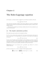
A <strong>FETI</strong>-<strong>DP</strong> FORMULATION FOR THE STOKES PROBLEM 7ΩΩ1 2λ 12λ 23λ 41Ω4λ13λ 24λ 34Ω3FIG. 1. Example <strong>of</strong> fully redundant Lagrange multipliers: λ 12 , λ 23 , λ 34 , and λ 41 are Lagrange multipliersused to en<strong>for</strong>ce continuity over common (closed) edges, and λ 13 and λ 24 are Lagrange multipliers used to en<strong>for</strong>cecontinuity among <strong>the</strong> subdomains sharing only <strong>the</strong> common vertex.number bound, CH/h, was obtained <strong>for</strong> elliptic problems with a choice <strong>of</strong> <strong>primal</strong> <strong>unknowns</strong>which are averages over common edges.Motivated by this fact, we will consider a set <strong>of</strong> <strong>primal</strong> velocity <strong>unknowns</strong>, which areaverages <strong>of</strong> <strong>the</strong> velocity <strong>unknowns</strong> on subdomain edges. In this case, <strong>the</strong> space ˜X consists <strong>of</strong><strong>the</strong> velocity <strong>unknowns</strong> that can be discontinuous at subdomain vertices and across subdomainedges except that <strong>the</strong>ir averages over common edges are <strong>the</strong> same. We will show that such achoice <strong>of</strong> <strong>primal</strong> <strong>unknowns</strong> gives an improved condition number bound,κ(̂M −1 F <strong>DP</strong> ) ≤ CH/h,compared to <strong>the</strong> previous choice <strong>of</strong> <strong>the</strong> <strong>primal</strong> velocity <strong>unknowns</strong> at subdomain vertices.3. Primal <strong>unknowns</strong> based on edge averages. In this section, we will provide an analysis<strong>of</strong> <strong>the</strong> condition number bound <strong>for</strong> <strong>the</strong> <strong>FETI</strong>-<strong>DP</strong> algorithm with a new set <strong>of</strong> <strong>primal</strong><strong>unknowns</strong>. Most part <strong>of</strong> <strong>the</strong> analysis can be done similarly to our previous work [5].We first describe <strong>the</strong> <strong>FETI</strong>-<strong>DP</strong> algorithm with such a <strong>selection</strong> <strong>of</strong> <strong>the</strong> <strong>primal</strong> <strong>unknowns</strong>.Differently to <strong>the</strong> <strong>primal</strong> <strong>unknowns</strong> at subdomain vertices, <strong>the</strong> velocity space ˜X has its elementsthat can be discontinuous at subdomain vertices. We introduce fully redundant Lagrangemultipliers to en<strong>for</strong>ce <strong>the</strong> continuity across Γ ij , see Figure 1,u (i)∆ − u(j) ∆ = 0,and our analysis is based on <strong>the</strong> fully redundant Lagrange multipliers.We note that <strong>the</strong> resulting <strong>FETI</strong>-<strong>DP</strong> equations have <strong>the</strong> null space which has more thanone dimension. In a more detail, F <strong>DP</strong> is positive definite on M c which is define byM c = { λ ∈ M : λ ⊥ Null(J T ∆) and λ T µ 0 = 0 } .Here Null(J T ∆ ) is <strong>the</strong> space <strong>of</strong> null components <strong>of</strong> J T ∆ and µ 0 is introduced in (2.11). Thenull components in Null(J∆ T ) are caused by <strong>the</strong> use <strong>of</strong> <strong>the</strong> fully redundant Lagrange multipli-
8 H.H. Kim, C.-O. Lee, and E.-H. Parkers. All <strong>the</strong>se components can be removed by <strong>the</strong> l 2 -orthogonal projection on M c . We <strong>the</strong>nper<strong>for</strong>m <strong>the</strong> conjugate gradient iteration on <strong>the</strong> subspace by projecting <strong>the</strong> residuals on M c .The o<strong>the</strong>r part <strong>of</strong> <strong>the</strong> <strong>FETI</strong>-<strong>DP</strong> algorithm is <strong>the</strong> same as in <strong>the</strong> previous section.We recall <strong>the</strong> enriched <strong>primal</strong> velocity space introduced in [5],Ê Π ={v ∈ ̂X}: v minimizes <strong>the</strong> discrete H 1 -seminorm <strong>for</strong> given values a V , a E .Here a Vand a E denote <strong>the</strong> given values <strong>of</strong> v at <strong>the</strong> subdomain vertices V and <strong>the</strong> givenaverage values <strong>of</strong> v on subdomain edges E, respectively. The pair <strong>of</strong> velocity and pressurespaces, (X I + ÊΠ, P ), is <strong>the</strong>n inf-sup stable with a constant β, which does not depend on anymesh parameters, see [5, Lemma 3.5].LetÊ I,Π = X I + ÊΠ.We will provide a condition number bound by proving <strong>the</strong> following inequalities:C 1 β 2 〈̂Mλ, λ〉 ≤ 〈F <strong>DP</strong> λ, λ〉 ≤ C 2Hh 〈̂Mλ, λ〉, ∀λ ∈ M c ,where β is <strong>the</strong> inf-sup constant <strong>of</strong> <strong>the</strong> pair (ÊI,Π, P ). These inequalities <strong>the</strong>n lead to <strong>the</strong>desired condition number boundκ(̂M −1 F <strong>DP</strong> ) ≤ C 1β 2 Hh .3.1. Lower bound analysis. Let N (x) be <strong>the</strong> set <strong>of</strong> subdomain indices sharing <strong>the</strong> pointx. We introduce an average operator,E ∆ w ∆ (x)| ∂Ωi =1|N (x)|∑j∈N (x)w (j)∆ (x),where |N (x)| is <strong>the</strong> number <strong>of</strong> elements in N (x). We <strong>the</strong>n have <strong>the</strong> identity,1(3.1) w ∆ (x)| ∂Ωi= E ∆ w ∆ (x)| ∂Ωi+|N (x)| J ∆J T ∆ w ∆ (x)∣ ,∂ΩisinceJ T ∆J ∆ w ∆ (x)| ∂Ωi = ∑(w (i)∆j∈N (x)(x) − w(j)∆ (x)).We introduce <strong>the</strong> matrix K which gives <strong>the</strong> discrete H 1 -seminorm on u ∈ ˜X, i.e.,N∑〈Ku, u〉 = |u| 2 H 1 (Ω i ) .LEMMA 3.1. For any µ ∈ M c , <strong>the</strong>re exists u ∈ ˜X such that1. J ∆ u ∆ = µ,i=1
A <strong>FETI</strong>-<strong>DP</strong> FORMULATION FOR THE STOKES PROBLEM 92. ∑ ∫i Ω i∇ · u q dx = 0, ∀q ∈ P,3. 〈Ku, u〉 ≤ C 1β〈K 2 ∆∆ J∆ T J ∆u ∆ , J∆ T J ∆u ∆ 〉, where β is <strong>the</strong> inf-sup constant <strong>of</strong> <strong>the</strong> pair(ÊI,Π, P ) and u ∆ is <strong>the</strong> part <strong>of</strong> dual <strong>unknowns</strong> <strong>of</strong> u.Pro<strong>of</strong>. Most part <strong>of</strong> <strong>the</strong> pro<strong>of</strong> is identical to [5, Lemma 4.2]. For a given µ ∈ M c , weselect w ∆ to satisfy(3.2) J ∆ w ∆ = µ and E ∆ w ∆ = 0.Similarly to <strong>the</strong> pro<strong>of</strong>s in [5], from such a w ∆ we can find u ∈ ˜X which satisfies <strong>the</strong> firsttwo conditions and〈Ku, u〉 ≤ C 1β 2 〈K ∆∆w ∆ , w ∆ 〉.From <strong>the</strong> above bound combined with (3.1), (3.2), and J ∆ u ∆ = J ∆ w ∆ , <strong>the</strong> third requirementon u <strong>the</strong>n follows.REMARK 3.2. In <strong>the</strong> above Lemma, w ∆ in (3.2) can be constructed as follows. SinceM c ⊂ Range(J ∆ ), <strong>for</strong> a given µ ∈ M c <strong>the</strong>re exists v ∆ ∈ ˜X such thatJ ∆ v ∆ = µ.For <strong>the</strong> v ∆ , we can find z ∆ ∈ ̂X which gives thatE ∆ (v ∆ + z ∆ ) = 0.Since z ∆ ∈ ̂X is continuous across <strong>the</strong> subdomain interface, J ∆ z ∆ = 0. We <strong>the</strong>n obtainw ∆ = v ∆ + z ∆ .We introduce∫(3.3) ˜X(div) ={v ∈ ˜X : ∇ · vq dx = 0Ω iWe <strong>the</strong>n have <strong>the</strong> identity,(3.4) 〈F <strong>DP</strong> λ, λ〉 = maxv∈ ˜X(div)where v ∆ is <strong>the</strong> part <strong>of</strong> dual <strong>unknowns</strong> <strong>of</strong> v.〈J ∆ v ∆ , λ〉 2,〈Kv, v〉}∀q ∈ P .By using Lemma 3.1 and (3.4) we obtain <strong>the</strong> lower bound, see [5, Theorem 4.3]:THEOREM 3.3. For any λ ∈ M c , we haveC 1 β 2 〈̂Mλ, λ〉 ≤ 〈F <strong>DP</strong> λ, λ〉,where β is <strong>the</strong> inf-sup constant <strong>of</strong> <strong>the</strong> pair (ÊI,Π, P ) and C 1 is a positive constant that doesnot depend on any mesh parameters.
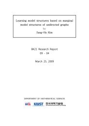
10 H.H. Kim, C.-O. Lee, and E.-H. Park3.2. Upper bound analysis. For a given edge E, let θ E denote <strong>the</strong> cut-<strong>of</strong>f functionwhich is one inside E and is zero, o<strong>the</strong>rwise. Similarly, we define <strong>the</strong> cut-<strong>of</strong>f function θ Vrelated to a vertex V . We need <strong>the</strong> following result <strong>for</strong> <strong>the</strong> upper bound analysis, see [13,Lemma 4] <strong>for</strong> <strong>the</strong> pro<strong>of</strong>:LEMMA 3.4. Let Ω i be a two dimensional subdomain. For any u (i) ∈ X (i) ,‖u (i) − c E ‖ 2 L 2 (E) ≤ CH|u(i) | 2 H 1 (Ω i ) ,where E is an edge <strong>of</strong> <strong>the</strong> subdomain Ω i and c E is given byc E =∫E Ih (θ E u (i) ) dx(s)∫E dx(s) .LEMMA 3.5. There exists a constant C such that <strong>for</strong> any u ∈ ˜X,where u ∆ is <strong>the</strong> part <strong>of</strong> dual <strong>unknowns</strong> <strong>of</strong> u.〈K ∆∆ J∆J T ∆ u ∆ , J∆J T ∆ u ∆ 〉 ≤ C H 〈Ku, u〉,hPro<strong>of</strong>. Let w ∆ = J T ∆ J ∆u ∆ . We note thatFrom <strong>the</strong> inverse inequality andwe obtain〈K ∆∆ J T ∆J ∆ u ∆ , J T ∆J ∆ u ∆ 〉 =N∑i=1|w (i)∆ |2 H 1 (Ω i) .‖w (i)∆ ‖2 L 2 (Ω i ) ≤ Ch‖w(i) ∆ ‖2 L 2 (∂Ω i ) ,(3.5) 〈K ∆∆ J T ∆J ∆ u ∆ , J T ∆J ∆ u ∆ 〉 ≤ Ch −1 N ∑We note that <strong>for</strong> x ∈ ∂Ω i(3.6) w (i)∆ (x) = ⎧⎨⎩u (i)∆∑m∈N (x)(x) − u(j)( ∆ (x),u (i)∆i=1‖w (i)∆ ‖2 L 2 (∂Ω i ) .)when x ∈ E ij,(x) − u(m)∆ (x) , when x ∈ V(∂Ω i ),where E ij is an open edge <strong>of</strong> Ω i , which is <strong>the</strong> common part <strong>of</strong> two subdomains Ω i and Ω j ,and V(∂Ω i ) is <strong>the</strong> set <strong>of</strong> vertices <strong>of</strong> Ω i . We decompose w (i)∆into(3.7) w (i)∆ = ∑I h (θ Eij w (i)∆ ) +E ij ⊂∂Ω iand <strong>the</strong>n compute each part using <strong>the</strong> <strong>for</strong>mula (3.6).∑V ∈V(∂Ω i)I h (θ V w (i)∆ )
A <strong>FETI</strong>-<strong>DP</strong> FORMULATION FOR THE STOKES PROBLEM 11v00 1100 1100 11ΩEkmm0000000000011111111111Ωi00 1100 1100 1100 1100 1100 1100 1100 1100 1100 1100 1100 1100 1100 1100 1100 1100 1100 1100 1100 1100 1100 1100 1100 1100 1100 1100 11EikΩkFIG. 2. Example <strong>of</strong> a path <strong>of</strong> subdomains sharing <strong>the</strong> vertex V : E ik and E km are edges connecting <strong>the</strong>subdomains in <strong>the</strong> path.For <strong>the</strong> first term <strong>of</strong> <strong>the</strong> above equation, by Lemma 3.4 we obtain(3.8)where‖I h (θ Eij w (i)∆ )‖2 L 2 (∂Ω i) = ‖Ih (θ Eij w (i)∆ )‖2 L 2 (E ij)≤ C‖u (i)∆ − u(j) ∆ ‖2 L 2 (E ij )= C‖u (i) − u (j) ‖ 2 L 2 (E ij)()≤ C ‖u (i) − c Eij ‖ 2 L 2 (E + ij) ‖u(j) − c Eij ‖ 2 L 2 (E ij)()≤ CH |u (i) | 2 H 1 (Ω i ) + |u(j) | 2 H 1 (Ω j ) ,∫∫Ec Eij =ijI h (θ Eij u (i) ) dx(s)E∫=ijI h (θ Eij u (j) ) dx(s)∫.dx(s)dx(s)E ijE ijWe note that u = (u (1) , · · · , u (N) ) ∈ ˜X, which has common edge averages across each E ij .For <strong>the</strong> term given at a vertex V , we consider subdomains in N (V ), which share <strong>the</strong>vertex V . Among <strong>the</strong>m, we select a path from Ω i to Ω m , {Ω i , Ω k1 , · · · , Ω kn , Ω m }, which areconnected through <strong>the</strong>ir common edges. We may assume that <strong>the</strong> path consists <strong>of</strong> {Ω i , Ω k , Ω m },see Figure 2. The following can also be applied to a more general case.At <strong>the</strong> vertex V ∈ V(∂Ω i ), we <strong>the</strong>n have that(3.9)‖I h (θ V w (i)∆ )‖2 L 2 (∂Ω i)≤ Ch∑≤ C≤ C≤ CHm∈N (V )∑m∈N (V )∑m∈N (V )∑(m∈N (V )|u (i)∆h|u (i)∆(V ) − u(m)∆(V )|2(V ) − u(k)∆ (V )|2 + h|u (k)∆(V ) − u(m)∆(V )|2)()‖u (i)∆ − u(k) ∆ ‖2 L 2 (E ik ) + ‖u(k) ∆− u(m) ∆ ‖2 L 2 (E km )()|u (i) | 2 H 1 (Ω + i) |u(k) | 2 H 1 (Ω k ) + |u(m) | 2 H 1 (Ω m) .
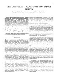
12 H.H. Kim, C.-O. Lee, and E.-H. ParkHere we have used <strong>the</strong> fact that both E ik and E km contain <strong>the</strong> vertex V and <strong>the</strong> inequalityused in (3.8). Note that E denotes <strong>the</strong> closure <strong>of</strong> an open edge E. Combining (3.5) with (3.7),(3.8), and (3.9), and usingN∑|u (i) | 2 1,Ω i= 〈Ku, u〉,i=1<strong>the</strong> desired bound has been proved.4.5]:From <strong>the</strong> identity in (3.4) and Lemma 3.5, an upper bound <strong>the</strong>n follows, see [5, LemmaTHEOREM 3.6. For any λ ∈ M c , we have〈F <strong>DP</strong> λ, λ〉 ≤ C 2Hh 〈̂Mλ, λ〉,where C 2 is a positive constant that does not depend on any mesh parameters.4. Numerical results. In this section, we provide numerical results <strong>of</strong> <strong>the</strong> <strong>FETI</strong>-<strong>DP</strong> algorithmscorresponding to <strong>the</strong> choice <strong>of</strong> <strong>primal</strong> <strong>unknowns</strong>. In <strong>the</strong> first choice, <strong>the</strong> velocity<strong>unknowns</strong> at subdomain vertices are selected and in <strong>the</strong> second <strong>the</strong> <strong>unknowns</strong> related to <strong>the</strong>velocity averages on common edges are selected. In <strong>the</strong> second case, we use <strong>the</strong> fully redundantLagrange multipliers to en<strong>for</strong>ce <strong>the</strong> continuity at <strong>the</strong> remaining dual velocity <strong>unknowns</strong>across <strong>the</strong> subdomain interface.We will present <strong>the</strong> number <strong>of</strong> iterations and approximated condition numbers <strong>of</strong> <strong>the</strong> two<strong>FETI</strong>-<strong>DP</strong> algorithms to confirm <strong>the</strong> bound <strong>of</strong> <strong>the</strong> condition number carried out in <strong>the</strong> previoussection. The conjugate gradient iteration is per<strong>for</strong>med up to <strong>the</strong> relative residual norm reducedby a factor <strong>of</strong> 10 6 and <strong>the</strong> condition numbers are approximated by <strong>the</strong> extreme eigenvalues <strong>of</strong><strong>the</strong> tridiagonal Lanczos matrix generated by <strong>the</strong> iteration. Our test problem is defined in <strong>the</strong>unit rectangular domain [0, 1] 2 with <strong>the</strong> exact solution,( )sin 3 (πx) sin 2 (πy) cos(πy)u(x, y) =and p(x, y) = x 2 − y 2 .− sin 2 (πx) sin 3 (πy) cos(πx)In Table 1, <strong>the</strong> results are presented as increasing <strong>the</strong> number <strong>of</strong> subdomains with a fixedlocal problem size in each subdomain. The domain is partitioned into uni<strong>for</strong>m rectangularsubdomains. For example, N = 4 2 means that <strong>the</strong> domain Ω is divided into four subdomainsin each x- and y-directional edges <strong>of</strong> Ω. The first choice <strong>of</strong> <strong>primal</strong> <strong>unknowns</strong> and <strong>the</strong> secondchoice <strong>of</strong> <strong>the</strong> <strong>primal</strong> <strong>unknowns</strong> are denoted by vertex-based and edge-based, respectively.For <strong>the</strong> both cases, <strong>the</strong> number <strong>of</strong> iterations and condition numbers do not depend on <strong>the</strong>number <strong>of</strong> subdomains. In o<strong>the</strong>r words, <strong>the</strong> results shows a good scalability with respect to<strong>the</strong> number <strong>of</strong> subdomains. For <strong>the</strong> second choice, we observe slightly less iterations andsmaller condition numbers.In Table 2, <strong>the</strong> number <strong>of</strong> iterations and condition numbers <strong>of</strong> <strong>the</strong> two choices are presentedas increasing <strong>the</strong> size <strong>of</strong> local problems. Here <strong>the</strong> domain Ω is divided into uni<strong>for</strong>m
A <strong>FETI</strong>-<strong>DP</strong> FORMULATION FOR THE STOKES PROBLEM 13vertex-basededge-basedN Iter κ λ min λ max Iter κ λ min λ max2 2 9 4.31e+00 2.60 1.12e+01 11 8.90 2.63 2.34e+014 2 16 1.17e+01 2.55 2.98e+01 18 1.05e+01 2.60 2.72e+018 2 21 1.36e+01 2.50 3.42e+01 20 1.16e+01 2.53 2.93e+0112 2 21 1.40e+01 2.50 3.50e+01 19 1.18e+01 2.51 2.98e+0116 2 22 1.41e+01 2.49 3.52e+01 19 1.19e+01 2.50 2.97e+01TABLE 1Scalability as increase <strong>of</strong> <strong>the</strong> number <strong>of</strong> subdomains, N, with a fixed local problem size (H/h = 8): <strong>the</strong>number <strong>of</strong> iterations Iter, <strong>the</strong> condition numbers κ, <strong>the</strong> minimum eigenvalues λ min , and <strong>the</strong> maximum eigenvaluesλ max <strong>of</strong> <strong>the</strong> vertex-based <strong>primal</strong> <strong>unknowns</strong> (<strong>the</strong> velocity values at <strong>the</strong> subdomain vertices are selected as <strong>the</strong><strong>primal</strong> <strong>unknowns</strong>) and <strong>the</strong> edge-based one (<strong>the</strong> averages <strong>of</strong> velocity over common edges are selected as <strong>the</strong> <strong>primal</strong><strong>unknowns</strong>)rectangular subdomains with N = 4 2 . The results from <strong>the</strong> second choice present weakerincrease <strong>of</strong> iterations and condition numbers as <strong>the</strong> increase <strong>of</strong> <strong>the</strong> local problem size, H/h,compared to those from <strong>the</strong> first choice. As in <strong>the</strong> analysis, <strong>the</strong> minimum eigenvalues arealmost identical <strong>for</strong> <strong>the</strong> both cases and do not depend on <strong>the</strong> size <strong>of</strong> local problems. <strong>On</strong>ly<strong>the</strong> maximum eigenvalues increase with respect to <strong>the</strong> size <strong>of</strong> local problems and <strong>the</strong> secondchoice gives less increase in <strong>the</strong> maximum eigenvalues than <strong>the</strong> first choice. In Figure 3, <strong>the</strong>constant C in <strong>the</strong> bound <strong>of</strong> condition numbers <strong>for</strong> <strong>the</strong> second choice,κ(M −1 F <strong>DP</strong> ) ≤ C H h ,is estimated as H/h increases. We observe that <strong>the</strong> estimated values <strong>of</strong> C tend to converge tosome number as H/h increases. The numerical results confirm that <strong>the</strong> bound <strong>of</strong> conditionnumbers are sharp.The second choice <strong>of</strong> <strong>primal</strong> <strong>unknowns</strong> based on subdomain edges shows better per<strong>for</strong>mancethan <strong>the</strong> first choice based on <strong>the</strong> subdomain vertices. The only complication in <strong>the</strong>second choice is introduction <strong>of</strong> additional null space components <strong>of</strong> <strong>the</strong> <strong>FETI</strong>-<strong>DP</strong> operatorcaused by using fully redundant Lagrange multipliers. This additional null space componentscan be eliminated by projecting <strong>the</strong> residual at each iteration. It is more practical to use <strong>the</strong>second choice <strong>of</strong> <strong>primal</strong> <strong>unknowns</strong> especially when <strong>the</strong> size <strong>of</strong> local problems are relativelylarge.REFERENCES[1] C. FARHAT, M. LESOINNE, P. LETALLEC, K. PIERSON, AND D. RIXEN, <strong>FETI</strong>-<strong>DP</strong>: a dual-<strong>primal</strong> unified<strong>FETI</strong> method. I. A faster alternative to <strong>the</strong> two-level <strong>FETI</strong> method, Internat. J. Numer. Methods Engrg.,50 (2001), pp. 1523–1544.
14 H.H. Kim, C.-O. Lee, and E.-H. Parkvertex-basededge-basedH/h Iter κ λ min λ max Iter κ λ min λ max4 12 5.09e+00 2.64 1.34e+01 15 7.17 3.23 2.32e+018 16 1.17e+01 2.55 2.98e+01 18 1.05e+01 2.59 2.72e+0116 24 2.78e+01 2.54 7.08e+01 21 1.31e+01 2.58 3.38e+0120 26 3.64e+01 2.57 9.36e+01 21 1.43e+01 2.59 3.72e+0126 29 5.04e+01 2.58 1.30e+02 22 1.62e+01 2.61 4.23e+0132 32 6.51e+01 2.59 1.68e+02 24 1.84e+01 2.60 4.79e+01TABLE 2Per<strong>for</strong>mance as increase <strong>of</strong> <strong>the</strong> size <strong>of</strong> local problems, H/h, in a fixed subdomain partition (N = 4 2 ): <strong>the</strong>number <strong>of</strong> iterations Iter, <strong>the</strong> condition numbers κ, <strong>the</strong> minimum eigenvalues λ min , and <strong>the</strong> maximum eigenvaluesλ max <strong>of</strong> <strong>the</strong> vertex-based <strong>primal</strong> <strong>unknowns</strong> (<strong>the</strong> velocity values at <strong>the</strong> subdomain vertices are selected as <strong>the</strong><strong>primal</strong> <strong>unknowns</strong>) and <strong>the</strong> edge-based one (<strong>the</strong> averages <strong>of</strong> velocity over common edges are selected as <strong>the</strong> <strong>primal</strong><strong>unknowns</strong>)2Estimated C=κ/(H/h)1.81.61.41.210.80.60.40 10 20 30 40 50 60 70H/h (local problem size)FIG. 3. Plot <strong>of</strong> estimated constant C = κ/(H/h) with respect to H/h <strong>for</strong> <strong>the</strong> edge-based <strong>primal</strong> <strong>unknowns</strong>[2] H. H. KIM, A <strong>FETI</strong>-<strong>DP</strong> <strong>for</strong>mulation <strong>of</strong> three dimensional elasticity problems with mortar discretization,SIAM J. Numer. Anal., 46 (2008), pp. 2346–2370.[3] H. H. KIM AND C.-O. LEE, A preconditioner <strong>for</strong> <strong>the</strong> <strong>FETI</strong>-<strong>DP</strong> <strong>for</strong>mulation with mortar methods in twodimensions, SIAM J. Numer. Anal., 42 (2005), pp. 2159–2175.[4] , A Neumann-Dirichlet preconditioner <strong>for</strong> a <strong>FETI</strong>-<strong>DP</strong> <strong>for</strong>mulation <strong>of</strong> <strong>the</strong> two-dimensional Stokes problemwith mortar methods, SIAM J. Sci. Comput., 28 (2006), pp. 1133–1152.[5] H. H. KIM, C.-O. LEE, AND E.-H. PARK, A <strong>FETI</strong>-<strong>DP</strong> <strong>for</strong>mulation <strong>for</strong> <strong>the</strong> Stokes problem without <strong>primal</strong>pressure components, Applied Ma<strong>the</strong>matics Research Report 08-04, KAIST, (2008).[6] A. KLAWONN AND O. RHEINBACH, Inexact <strong>FETI</strong>-<strong>DP</strong> methods, Inter. J. Numer. Methods Engrg., 69 (2007),pp. 284–307.[7] A. KLAWONN AND O. B. WIDLUND, Dual-<strong>primal</strong> <strong>FETI</strong> methods <strong>for</strong> linear elasticity, Comm. Pure Appl.Math., 59 (2006), pp. 1523–1572.[8] A. KLAWONN, O. B. WIDLUND, AND M. DRYJA, Dual-<strong>primal</strong> <strong>FETI</strong> methods <strong>for</strong> three-dimensional ellipticproblems with heterogeneous coefficients, SIAM J. Numer. Anal., 40 (2002), pp. 159–179.[9] J. LI, Dual-<strong>primal</strong> <strong>FETI</strong> methods <strong>for</strong> stationary Stokes and Navier-Stokes equations, Ph. D. Thesis, Depart-
A <strong>FETI</strong>-<strong>DP</strong> FORMULATION FOR THE STOKES PROBLEM 15ment <strong>of</strong> Ma<strong>the</strong>matics, Courant Institute, New York University, 2002.[10] , A dual-<strong>primal</strong> <strong>FETI</strong> method <strong>for</strong> incompressible Stokes equations, Numer. Math., 102 (2005), pp. 257–275.[11] J. LI AND O. WIDLUND, BDDC algorithms <strong>for</strong> incompressible Stokes equations, SIAM J. Numer. Anal., 44(2006), pp. 2432–2455.[12] J. LI AND O. B. WIDLUND, <strong>FETI</strong>-<strong>DP</strong>, BDDC, and block Cholesky methods, Internat. J. Numer. MethodsEngrg., 66 (2006), pp. 250–271.[13] , <strong>On</strong> <strong>the</strong> use <strong>of</strong> inexact subdomain solvers <strong>for</strong> BDDC algorithms, Comput. Methods Appl. Mech.Engrg., 196 (2007), pp. 1415–1428.[14] L. F. PAVARINO AND O. B. WIDLUND, Balancing Neumann-Neumann methods <strong>for</strong> incompressible Stokesequations, Comm. Pure Appl. Math., 55 (2002), pp. 302–335.