Model Selection Based on the Modulus of Continuity
Model Selection Based on the Modulus of Continuity
Model Selection Based on the Modulus of Continuity

Create successful ePaper yourself
Turn your PDF publications into a flip-book with our unique Google optimized e-Paper software.
<strong>the</strong> trade-<strong>of</strong>f between <strong>the</strong> under-fitting and over-fitting <strong>of</strong> regressi<strong>on</strong> models. Here, <strong>the</strong> importantissue is measuring <strong>the</strong> model complexity related to <strong>the</strong> variance term. The statisticalmethods <strong>of</strong> model selecti<strong>on</strong> is to use a penalty (correcti<strong>on</strong>) factor as <strong>the</strong> measure <strong>of</strong> modelcomplexity. The well known criteria are Akaike informati<strong>on</strong> criteria (AIC)[1], Bayesian informati<strong>on</strong>criteria (BIC)[2], generalized cross-validati<strong>on</strong> (GCV)[3], minimum descripti<strong>on</strong> length(MDL)[4, 5], and risk inflati<strong>on</strong> criteria (RIC)[6]. These methods can be easily fit to linearregressi<strong>on</strong> models when <strong>the</strong> large number <strong>of</strong> samples is available. However, <strong>the</strong>y suffer <strong>the</strong>difficulty to select <strong>the</strong> optimal structure <strong>of</strong> <strong>the</strong> estimati<strong>on</strong> networks in <strong>the</strong> case <strong>of</strong> n<strong>on</strong>linearregressi<strong>on</strong> models and/or <strong>the</strong> small number <strong>of</strong> samples. Recently, Vapnik[7] proposed <strong>the</strong>model selecti<strong>on</strong> method based <strong>on</strong> <strong>the</strong> structural risk minimizati<strong>on</strong> (SRM) principle. One <strong>of</strong>characteristics <strong>of</strong> this method is that <strong>the</strong> model complexity is described by <strong>the</strong> structuralinformati<strong>on</strong> such as <strong>the</strong> VC dimensi<strong>on</strong> <strong>of</strong> <strong>the</strong> estimati<strong>on</strong> network. This method can be appliedto <strong>the</strong> n<strong>on</strong>linear models and also <strong>the</strong> regressi<strong>on</strong> models using small number <strong>of</strong> samples.Chapelle et al.[8] and Cherkasky et al.[9] showed that <strong>the</strong> SRM based model selecti<strong>on</strong> is ableto outperform o<strong>the</strong>r statistical methods such as AIC or BIC. These methods require <strong>the</strong>actual VC dimensi<strong>on</strong> <strong>of</strong> <strong>the</strong> hypo<strong>the</strong>sis space associated with <strong>the</strong> estimati<strong>on</strong> network, whichis not easy to determine in <strong>the</strong> case <strong>of</strong> n<strong>on</strong>linear regressi<strong>on</strong> models.In this paper, we present <strong>the</strong> risk functi<strong>on</strong> bounds in <strong>the</strong> sense <strong>of</strong> <strong>the</strong> modulus <strong>of</strong> c<strong>on</strong>tinuity(MC) representing a measure <strong>of</strong> c<strong>on</strong>tinuity for <strong>the</strong> given functi<strong>on</strong>. Lorentz[10] applied <strong>the</strong> MCto <strong>the</strong> functi<strong>on</strong> approximati<strong>on</strong> <strong>the</strong>ories. In our method, this measure is applied to determine<strong>the</strong> risk functi<strong>on</strong> bounds in <strong>the</strong> L 1 sense. For <strong>the</strong> estimati<strong>on</strong> <strong>of</strong> <strong>the</strong>se bounds, <strong>the</strong> MC isanalyzed for both <strong>the</strong> target and estimati<strong>on</strong> functi<strong>on</strong>s. As a result, <strong>the</strong> suggested boundsinclude both <strong>the</strong> structural informati<strong>on</strong> such as <strong>the</strong> number <strong>of</strong> parameters and <strong>the</strong> learnedresults such as <strong>the</strong> weight values <strong>of</strong> <strong>the</strong> estimati<strong>on</strong> network. Through <strong>the</strong> simulati<strong>on</strong> forfuncti<strong>on</strong> approximati<strong>on</strong>, we have shown that <strong>the</strong> MC based method can provide <strong>the</strong> better2
Example: C<strong>on</strong>sider <strong>the</strong> trig<strong>on</strong>ometric polynomials φ 0 (x) = 1/2, φ 2j−1 (x) = sin jx, andφ 2j (x) = cos jx for j = 1, 2, · · · , n. Applying <strong>the</strong> mean value <strong>the</strong>orem to φ j , we getω(φ k , h) ‖φ ′ k‖ ∞ h n · h for k = 0, · · · , 2n.That is,max {ω(φ k, h)} n · h.0k2nTherefore, <strong>the</strong> upper bounds <strong>of</strong> risk functi<strong>on</strong>s can be determined byR(f n ) L1 R emp (f n ) L1 + ω(f, h) + n · h2n∑k=0|w k | + σ√2δ . (24)Similarly, we can derive <strong>the</strong> upper bounds <strong>of</strong> risk functi<strong>on</strong>s for <strong>the</strong> regressi<strong>on</strong> model usingalgebraic polynomials, that is, f n (x) = ∑ ni=0 w ix i .Example: C<strong>on</strong>sider <strong>the</strong> following form <strong>of</strong> radial basis functi<strong>on</strong>s:φ k (x) = exp(− (x − t )k) 22σ 2 kfor k = 1, · · · , nwhere t k and σ 2 k represent <strong>the</strong> center and width <strong>of</strong> <strong>the</strong> basis functi<strong>on</strong> φ k respectively.Applying <strong>the</strong> mean value <strong>the</strong>orem to φ k , we getω(φ k , h) ‖φ ′ k‖ ∞ h h (exp − 1 )σ k 2for k = 1, · · · , nsince φ ′ k has <strong>the</strong> maximum and minimum at x = t i − σ k and x = t i + σ k respectively.This implies thatmax {ω(φ k, h)} h (exp − 1 )1kn σ ′ 2whereσ ′ = min1kn σ k.9
Therefore, <strong>the</strong> upper bound <strong>of</strong> risk functi<strong>on</strong> can be determined byR(f n ) L1 R emp (f n ) L1 + ω(f, h) + h (exp − 1 ) n∑ 2|wσ ′ k | + σ√2δ . (25)k=1Example: C<strong>on</strong>sider <strong>the</strong> following form <strong>of</strong> sigmoid functi<strong>on</strong>s:φ k (x) =11 + exp(−a i x + b i )for k = 1, · · · , nwhere a k and b k represent <strong>the</strong> adaptable parameters <strong>of</strong> <strong>the</strong> basis functi<strong>on</strong> φ k . Applying<strong>the</strong> mean value <strong>the</strong>orem to φ k , we getw(φ k , h) ‖φ ′ k‖ ∞ h h 4for k = 1, · · · , nsince φ ′ k has <strong>the</strong> maximum at x = b k/a k . That is,max {ω(φ k, h)} h1kn 4 .Therefore, <strong>the</strong> upper bound <strong>of</strong> <strong>the</strong> risk functi<strong>on</strong>s can be determined byR(f n ) L1 R emp (f n ) L1 + ω(f, h) + h 4n∑ 2|w k | + σ√δ . (26)k=1The suggested <strong>the</strong>orem <strong>of</strong> true risk bounds is derived in <strong>the</strong> sense <strong>of</strong> <strong>the</strong> L 1 measure, that is,<strong>the</strong> risk functi<strong>on</strong> described by (16). O<strong>the</strong>r model selecti<strong>on</strong> criteria such as AIC and SEB arederived from <strong>the</strong> risk functi<strong>on</strong> using <strong>the</strong> quadratic loss functi<strong>on</strong> L(y, f n (x)) = (y −f n (x)) 2 . Inthis c<strong>on</strong>text, we can show that <strong>the</strong> optimal functi<strong>on</strong> f n ∗(x) determined from <strong>the</strong> risk functi<strong>on</strong><strong>of</strong> <strong>the</strong> L 1 measure is also optimal in <strong>the</strong> sense <strong>of</strong> <strong>the</strong> risk functi<strong>on</strong> using <strong>the</strong> quadratic lossfuncti<strong>on</strong> under <strong>the</strong> assumpti<strong>on</strong> that <strong>the</strong> estimati<strong>on</strong> functi<strong>on</strong> is unbiased and <strong>the</strong> error termy − f n (x) has normal distributi<strong>on</strong>.10
4 Simulati<strong>on</strong>The simulati<strong>on</strong> for functi<strong>on</strong> approximati<strong>on</strong> was performed using <strong>the</strong> regressi<strong>on</strong> model withtrig<strong>on</strong>ometric polynomial functi<strong>on</strong>s. In this regressi<strong>on</strong>, various model selecti<strong>on</strong> methods suchas <strong>the</strong> AIC, BIC, VC dimensi<strong>on</strong>, and MC based methods were tested. As <strong>the</strong> VC dimensi<strong>on</strong>based method, we choose <strong>the</strong> smallest eigenvalue based (SEB) method[8] suggested byChapelle et al. Here, <strong>the</strong> trig<strong>on</strong>ometric polynomial functi<strong>on</strong>s were selected as <strong>the</strong> basis functi<strong>on</strong>ssince this network could be c<strong>on</strong>sidered as <strong>the</strong> linear regressi<strong>on</strong> model so that <strong>the</strong> VCdimensi<strong>on</strong> <strong>of</strong> <strong>the</strong> network was easy to find out and <strong>the</strong> optimizati<strong>on</strong> <strong>of</strong> network parameterscould be easily solved. This makes easier to compare <strong>the</strong> suggested method with o<strong>the</strong>r methods.In this simulati<strong>on</strong>, <strong>the</strong> data (x i , y i ) were generated by (1). Here, <strong>the</strong> input value x i wereuniformly distributed within <strong>the</strong> interval <strong>of</strong> [−π, π]. As <strong>the</strong> target functi<strong>on</strong>s, <strong>the</strong> followingfuncti<strong>on</strong>s were used:1) <strong>the</strong> step functi<strong>on</strong> defined by⎧⎪⎨ 1 if x 0f(x) =⎪⎩ 0 o<strong>the</strong>rwise,(27)2) <strong>the</strong> sine square functi<strong>on</strong> defined byf(x) = sin 2 (x), (28)3) <strong>the</strong> sinc functi<strong>on</strong> defined by4) and <strong>the</strong> combined functi<strong>on</strong> defined byf(x) = sin(πx)πx , (29)f(x) = 2x exp(− x2) cos(2πx). (30)2The target functi<strong>on</strong>s were illustrated in Figure 1. The first target functi<strong>on</strong> was disc<strong>on</strong>tinuouswhile o<strong>the</strong>r functi<strong>on</strong>s were c<strong>on</strong>tinuous. The sec<strong>on</strong>d and third functi<strong>on</strong>s showed <strong>the</strong>11
similar complexity while <strong>the</strong> fourth functi<strong>on</strong> was more complex than o<strong>the</strong>r functi<strong>on</strong>s. For<strong>the</strong>se target functi<strong>on</strong>, we generated N (= 50) training samples randomly according to <strong>the</strong>target functi<strong>on</strong> to train <strong>the</strong> estimati<strong>on</strong> network. We also generated 300 test samples separately.For <strong>the</strong> estimati<strong>on</strong> network, <strong>the</strong> basis functi<strong>on</strong>s <strong>of</strong> trig<strong>on</strong>ometric polynomial networkwere given byφ 0 (x) = 1 2 , φ 2j−1(x) = sin jx, and φ 2j (x) = cos jx,where j represents <strong>the</strong> period <strong>of</strong> sinusoidal functi<strong>on</strong>. Here, <strong>the</strong> estimati<strong>on</strong> functi<strong>on</strong> f n (x) wasgiven byn∑f n (x) = w k φ k (x). (31)k=0For N samples, <strong>the</strong> observati<strong>on</strong> vector defined by y = (y 1 , · · · , y N ) T can be approximatedby <strong>the</strong> following vector form:y = Φ n w (32)where Φ n was a matrix in which <strong>the</strong> ij-th element was given by φ j (x i ) and w was a weightvector defined by w = (w 0 , · · · , w n ) T . From <strong>the</strong> empirical risk minimizati<strong>on</strong> <strong>of</strong> square lossfuncti<strong>on</strong>, <strong>the</strong> estimated weight vector ŵ could be determined byŵ = (Φ T nΦ n ) −1 Φ T ny. (33)By substituting <strong>the</strong> estimated weight vector to (32), we obtained <strong>the</strong> empirical risk R emp (f n )evaluated by <strong>the</strong> training samples and <strong>the</strong> estimated risk ̂R(f n ) could be determined by <strong>the</strong>AIC, BIC, SEB, and MC based methods. Here, <strong>the</strong> estimated optimal number <strong>of</strong> nodes wasdetermined bŷn = arg minn̂R(fn ). (34)Note that in <strong>the</strong> MC method, <strong>on</strong>ly <strong>the</strong> terms <strong>of</strong> R emp (f n ) and <strong>the</strong> modulus <strong>of</strong> c<strong>on</strong>tinuityfor <strong>the</strong> estimati<strong>on</strong> functi<strong>on</strong> were c<strong>on</strong>sidered to select <strong>the</strong> optimal number <strong>of</strong> nodes sinceo<strong>the</strong>r terms in (19) were c<strong>on</strong>stant <strong>on</strong>ce <strong>the</strong> training samples were given. To compare <strong>the</strong> risk12
functi<strong>on</strong>s obtained for <strong>the</strong> estimated optimal number <strong>of</strong> nodes ̂n with <strong>the</strong> risk functi<strong>on</strong>s for<strong>the</strong> minimum number <strong>of</strong> nodes obtained from <strong>the</strong> test samples, we computed <strong>the</strong> log ratio<strong>of</strong> two risks, that is,r R = logR(f̂n )min n R(f n )(35)where R(f n ) represented <strong>the</strong> risk functi<strong>on</strong> for <strong>the</strong> squared error loss functi<strong>on</strong> L(y, f n ) =(y − f n (x)) 2 . This risk ratio represented <strong>the</strong> quality <strong>of</strong> distance between <strong>the</strong> optimal and <strong>the</strong>estimated optimal risks. We also computed <strong>the</strong> log ratio <strong>of</strong> <strong>the</strong> estimated optimal number <strong>of</strong>nodes ̂n to <strong>the</strong> minimum number <strong>of</strong> nodes obtained from <strong>the</strong> test patterns, that is,r n = loĝnarg min n R(f n ) . (36)This node ratio represented <strong>the</strong> quality <strong>of</strong> distance between <strong>the</strong> optimal and <strong>the</strong> estimatedoptimal complexity <strong>of</strong> <strong>the</strong> network. After all experiments have been repeated 1000 times, <strong>the</strong>risk ratios <strong>of</strong> (35) and <strong>the</strong> node ratios <strong>of</strong> (36) were plotted using <strong>the</strong> box-plot method. Thesimulati<strong>on</strong> results <strong>of</strong> model selecti<strong>on</strong> using <strong>the</strong> AIC, BIC, SEB and MC based methods wereillustrated in Figures 2 through 9. These simulati<strong>on</strong> results showed us that 1) <strong>the</strong> SEB basedmethod outperformed <strong>the</strong> AIC and BIC based methods from <strong>the</strong> view point <strong>of</strong> risk ratiosin <strong>the</strong> case <strong>of</strong> <strong>the</strong> first, sec<strong>on</strong>d, and third target functi<strong>on</strong>s but not in <strong>the</strong> case <strong>of</strong> <strong>the</strong> fourthfuncti<strong>on</strong>, that is, more complicated functi<strong>on</strong>, 2) while <strong>the</strong> MC method dem<strong>on</strong>strated <strong>the</strong> toplevel performance from <strong>the</strong> view points <strong>of</strong> risk and node ratios for all four target functi<strong>on</strong>s.In general, <strong>the</strong> SEB method showed good performance when <strong>the</strong> ratio <strong>of</strong> <strong>the</strong> optimal number<strong>of</strong> nodes to <strong>the</strong> number <strong>of</strong> samples n ∗ /l was small since <strong>the</strong> true risk bounds based <strong>on</strong> <strong>the</strong> VCdimensi<strong>on</strong> were derived in <strong>the</strong> sense <strong>of</strong> uniform c<strong>on</strong>vergence, that is, <strong>the</strong> worst case in <strong>the</strong>hypo<strong>the</strong>sis space. As an example, we illustrated n ∗ /l for four target functi<strong>on</strong>s in Figure 10.As we expected, <strong>the</strong> fourth target functi<strong>on</strong> required high n ∗ /l compared to o<strong>the</strong>r targetfuncti<strong>on</strong>s due to <strong>the</strong> complexity <strong>of</strong> functi<strong>on</strong> as shown in Figure 1. In this case, <strong>the</strong> SEBmethod did not show good performance.13
To see <strong>the</strong> risk predicti<strong>on</strong> <strong>of</strong> <strong>the</strong> model selecti<strong>on</strong> methods, we plotted <strong>the</strong> estimated errorversus <strong>the</strong> number <strong>of</strong> nodes for <strong>the</strong> AIC, BIC, and SEB methods in <strong>the</strong> L 2 sense <strong>of</strong> lossfuncti<strong>on</strong>, that is, <strong>the</strong> square root <strong>of</strong> risk functi<strong>on</strong>, and also for <strong>the</strong> MC method in <strong>the</strong> L 1sense <strong>of</strong> loss functi<strong>on</strong> defined by (16). The predicted results were compared with test errors asshown in Figures 11 and 12. Theses results showed that 1) <strong>the</strong> risk predicti<strong>on</strong> using <strong>the</strong> AICand BIC methods fit well except <strong>the</strong> sudden change in risk functi<strong>on</strong>s, 2) <strong>the</strong> risk predicti<strong>on</strong>using <strong>the</strong> SEB method had <strong>the</strong> tendency to fit well when <strong>the</strong> ratio <strong>of</strong> <strong>the</strong> number <strong>of</strong> nodes to<strong>the</strong> number <strong>of</strong> samples n/l was small, and 3) <strong>the</strong> risk predicti<strong>on</strong> using <strong>the</strong> MC method waswell suited with <strong>the</strong> test errors in overall range <strong>of</strong> <strong>the</strong> number <strong>of</strong> nodes. In <strong>the</strong>se predictedresults, it was interesting that <strong>the</strong> MC method was able to catch <strong>the</strong> sudden change <strong>of</strong> testerrors while o<strong>the</strong>r methods didn’t.In summary, <strong>the</strong> performance <strong>of</strong> <strong>the</strong> MC based method showed <strong>the</strong> better performancefor various types <strong>of</strong> target functi<strong>on</strong>s from <strong>the</strong> view points <strong>of</strong> risk and node ratios compared too<strong>the</strong>r methods. We also dem<strong>on</strong>strated that <strong>the</strong> risk predicti<strong>on</strong> using <strong>the</strong> MC method was ableto catch <strong>the</strong> trend <strong>of</strong> test errors. This was mainly due to <strong>the</strong> fact that <strong>the</strong> MC based methodwas performed using <strong>the</strong> risk functi<strong>on</strong> bounds incorporating <strong>the</strong> informati<strong>on</strong> <strong>of</strong> learned resultssuch as <strong>the</strong> sum <strong>of</strong> absolute weights as well as <strong>the</strong> structural informati<strong>on</strong> <strong>of</strong> <strong>the</strong> estimati<strong>on</strong>network. Fur<strong>the</strong>rmore, <strong>the</strong> suggested MC method can be easily extended to various types <strong>of</strong>regressi<strong>on</strong> models with n<strong>on</strong>linear kernel functi<strong>on</strong>s which have some smoothness c<strong>on</strong>straints.14
10.80.60.40.20−4 −2 0 2 4(a) step10.80.60.40.20−4 −2 0 2 4(b) sin 2 (x)1.510.50−0.5−4 −2 0 2 4(c) sinc(x)1.510.50−0.5−1−1.5−4 −2 0 2 4(d) 2xexp(−x 2 )cos(2π x)Fig. 1. The target functi<strong>on</strong>s for <strong>the</strong> simulati<strong>on</strong> <strong>of</strong> model selecti<strong>on</strong>:15
32.521.510.50AIC BIC SEB MC(a)32.521.510.50AIC BIC SEB MC(b)32.521.510.50AIC BIC SEB MC(c)32.521.510.50AIC BIC SEB MC(d)Fig. 2. The box-plots <strong>of</strong> risk ratios r R for <strong>the</strong> regressi<strong>on</strong> <strong>of</strong> step functi<strong>on</strong>: (a), (b), (c), and (d) represent <strong>the</strong> box-plots<strong>of</strong> r R with σ = 0, 0.025, 0.05, and 0.1 respectively.16
21.510.50AIC BIC SEB MC(a)21.510.50AIC BIC SEB MC(b)21.510.50AIC BIC SEB MC(c)21.510.50AIC BIC SEB MC(d)Fig. 3. The box-plots <strong>of</strong> node ratios r n for <strong>the</strong> regressi<strong>on</strong> <strong>of</strong> step functi<strong>on</strong>: (a), (b), (c), and (d) represent <strong>the</strong> box-plots<strong>of</strong> r n with σ = 0, 0.025, 0.05, and 0.1 respectively.17
32.521.510.50AIC BIC SEB MC(a)32.521.510.50AIC BIC SEB MC(b)32.521.510.50AIC BIC SEB MC(c)32.521.510.50AIC BIC SEB MC(d)Fig. 4. The box-plots <strong>of</strong> risk ratios r R for <strong>the</strong> regressi<strong>on</strong> <strong>of</strong> sine-square functi<strong>on</strong>: (a), (b), (c), and (d) represent <strong>the</strong>box-plots <strong>of</strong> r R with σ = 0, 0.025, 0.05, and 0.1 respectively.18
21.510.50AIC BIC SEB MC(a)21.510.50AIC BIC SEB MC(b)21.510.50AIC BIC SEB MC(c)21.510.50AIC BIC SEB MC(d)Fig. 5. The box-plots <strong>of</strong> node ratios r n for <strong>the</strong> regressi<strong>on</strong> <strong>of</strong> sine-square functi<strong>on</strong>: (a), (b), (c), and (d) represent <strong>the</strong>box-plots <strong>of</strong> r n with σ = 0, 0.025, 0.05, and 0.1 respectively.19
32.521.510.50AIC BIC SEB MC(a)32.521.510.50AIC BIC SEB MC(b)32.521.510.50AIC BIC SEB MC(c)32.521.510.50AIC BIC SEB MC(d)Fig. 6. The box-plots <strong>of</strong> risk ratios r R for <strong>the</strong> regressi<strong>on</strong> <strong>of</strong> sinc functi<strong>on</strong>: (a), (b), (c), and (d) represent <strong>the</strong> box-plots<strong>of</strong> r R with σ = 0, 0.025, 0.05, and 0.1 respectively.20
21.510.50AIC BIC SEB MC(a)21.510.50AIC BIC SEB MC(b)21.510.50AIC BIC SEB MC(c)21.510.50AIC BIC SEB MC(d)Fig. 7. The box-plots <strong>of</strong> node ratios r n for <strong>the</strong> regressi<strong>on</strong> <strong>of</strong> sinc functi<strong>on</strong>: (a), (b), (c), and (d) represent <strong>the</strong> box-plots<strong>of</strong> r n with σ = 0, 0.025, 0.05, and 0.1 respectively.21
32.521.510.50AIC BIC SEB MC(a)32.521.510.50AIC BIC SEB MC(b)32.521.510.50AIC BIC SEB MC(c)32.521.510.50AIC BIC SEB MC(d)Fig. 8. The box-plots <strong>of</strong> risk ratios r R for <strong>the</strong> regressi<strong>on</strong> <strong>of</strong> combined functi<strong>on</strong>: (a), (b), (c), and (d) represent <strong>the</strong>box-plots <strong>of</strong> r R with σ = 0, 0.025, 0.05, and 0.1 respectively.22
21.510.50AIC BIC SEB MC(a)21.510.50AIC BIC SEB MC(b)21.510.50AIC BIC SEB MC(c)21.510.50AIC BIC SEB MC(d)Fig. 9. The box-plots <strong>of</strong> node ratios r n for <strong>the</strong> regressi<strong>on</strong> <strong>of</strong> combined functi<strong>on</strong>: (a), (b), (c), and (d) represent <strong>the</strong>box-plots <strong>of</strong> r n with σ = 0, 0.025, 0.05, and 0.1 respectively.23
0.80.60.40.20 0.025 0.05 0.1(a)0.80.60.40.20 0.025 0.05 0.1(b)0.80.60.40.20 0.025 0.05 0.1(c)0.80.60.40.200 0.025 0.05 0.1(d)Fig. 10. The box-plots for <strong>the</strong> optimal number <strong>of</strong> nodes to <strong>the</strong> number <strong>of</strong> samples n ∗ /l: (a), (b), (c), and (d) represent<strong>the</strong> box-plots <strong>of</strong> n ∗ /l in <strong>the</strong> regressi<strong>on</strong> <strong>of</strong> step, sine-square, sinc, and combined functi<strong>on</strong>s respectively.24
10.90.8train errortest errorBICSEBAIC0.70.60.50.40.30.20.100 5 10 15 20 25 30 35 40 45(a)10.9test errortrain errorMC0.80.70.60.50.40.30.20.100 5 10 15 20 25 30 35 40 45(b)Fig. 11. Performance Predicti<strong>on</strong>s <strong>of</strong> model selecti<strong>on</strong> methods in <strong>the</strong> case <strong>of</strong> sinc functi<strong>on</strong>: (a) represents <strong>the</strong> estimatederror in <strong>the</strong> L 2 sense versus <strong>the</strong> number <strong>of</strong> nodes using <strong>the</strong> AIC, BIC, and SEB methods and (b) represents <strong>the</strong>estimated error in <strong>the</strong> L 1 sense versus <strong>the</strong> number <strong>of</strong> nodes using <strong>the</strong> MC method.25
10.90.8train errortest errorBICSEBAIC0.70.60.50.40.30.20.100 5 10 15 20 25 30 35 40 45(a)10.9test errortrain errorMC0.80.70.60.50.40.30.20.100 5 10 15 20 25 30 35 40 45(b)Fig. 12. Performance Predicti<strong>on</strong>s <strong>of</strong> model selecti<strong>on</strong> methods in <strong>the</strong> case <strong>of</strong> combined functi<strong>on</strong>: (a) represents <strong>the</strong>estimated error in <strong>the</strong> L 2 sense versus <strong>the</strong> number <strong>of</strong> nodes using <strong>the</strong> AIC, BIC, and SEB methods and (b) represents<strong>the</strong> estimated error in <strong>the</strong> L 1 sense versus <strong>the</strong> number <strong>of</strong> nodes using <strong>the</strong> MC method.26
5 C<strong>on</strong>clusi<strong>on</strong>We have suggested a new method <strong>of</strong> model selecti<strong>on</strong> in regressi<strong>on</strong> problems based <strong>on</strong> <strong>the</strong>modulus <strong>of</strong> c<strong>on</strong>tinuity. The risk functi<strong>on</strong> bounds are investigated from <strong>the</strong> view point <strong>of</strong> <strong>the</strong>modulus <strong>of</strong> c<strong>on</strong>tinuity for both <strong>the</strong> target and estimati<strong>on</strong> functi<strong>on</strong>s. The final form <strong>of</strong> <strong>the</strong> riskfuncti<strong>on</strong> bounds incorporate <strong>the</strong> informati<strong>on</strong> <strong>of</strong> learned results such as <strong>the</strong> sum <strong>of</strong> absoluteweights as well as <strong>the</strong> structural informati<strong>on</strong> such as <strong>the</strong> number <strong>of</strong> nodes in <strong>the</strong> regressi<strong>on</strong>model. To verify <strong>the</strong> validity <strong>of</strong> <strong>the</strong> suggested bound, <strong>the</strong> model selecti<strong>on</strong> <strong>of</strong> regressi<strong>on</strong> modelsusing <strong>the</strong> trig<strong>on</strong>ometric polynomials in functi<strong>on</strong> approximati<strong>on</strong> problem was performed. Asa result, <strong>the</strong> suggested method showed <strong>the</strong> better performance for various types <strong>of</strong> targetfuncti<strong>on</strong>s from <strong>the</strong> view points <strong>of</strong> risk and node ratios compared to o<strong>the</strong>r model selecti<strong>on</strong>methods. We also dem<strong>on</strong>strated that <strong>the</strong> risk predicti<strong>on</strong> using <strong>the</strong> MC method was able tocatch <strong>the</strong> trend <strong>of</strong> test errors. This was mainly due to <strong>the</strong> fact that <strong>the</strong> MC based methodwas performed using <strong>the</strong> risk functi<strong>on</strong> bounds incorporating both <strong>the</strong> informati<strong>on</strong> <strong>of</strong> learnedresults as well as <strong>the</strong> structural informati<strong>on</strong> <strong>of</strong> <strong>the</strong> estimati<strong>on</strong> network, <strong>the</strong> main criteria<strong>of</strong> o<strong>the</strong>r model selecti<strong>on</strong> methods. Fur<strong>the</strong>rmore, <strong>the</strong> suggested MC method can be easilyextended to various types <strong>of</strong> regressi<strong>on</strong> models with n<strong>on</strong>linear kernel functi<strong>on</strong>s which havesome smoothness c<strong>on</strong>straints.27
References1. Akaike, H.: Informati<strong>on</strong> <strong>the</strong>ory and an extansi<strong>on</strong> <strong>of</strong> <strong>the</strong> maximum likelihood principle. In Petrov, B. and Csaki,F., editors, 2nd Interanati<strong>on</strong>al Symposium <strong>on</strong> Informati<strong>on</strong> Theory, VOL. 22 (1973), 267–281, Budapest.2. Schwartz, G.: Estimating <strong>the</strong> dimensi<strong>on</strong> <strong>of</strong> a model. Ann. Stat., 6 (1978),461–464.3. Wahba, G., Golub, G., and Heath, M.: Generalized cross-validati<strong>on</strong> as a method for choosing a good ridge parameter.Technometrics, 21 (1979), 215–223.4. Rissanen, J.: Stochastic complexity and modeling. Annals <strong>of</strong> Statistics, 14 (1986), 1080–1100.5. Barr<strong>on</strong>, A., Rissanen, J., and Yu, B.: The minimum descripti<strong>on</strong> length principle in coding and modeling. IEEETransacti<strong>on</strong>s <strong>on</strong> Infomati<strong>on</strong> Theory, 44 (1998), 2743–2760.6. Dean P. Foster and Edward I. George: The risk inflati<strong>on</strong> criteri<strong>on</strong> for multiple regressi<strong>on</strong>. Annals <strong>of</strong> Statistics, 22(1994), 1947–1975.7. Vladimir N. Vapnik: Statistical Learning Theory. J. Wiley, 19988. Olivier Chapelle, Vladimir Vapnik, Yoshua Bengio: <str<strong>on</strong>g>Model</str<strong>on</strong>g> selecti<strong>on</strong> for small sample regressi<strong>on</strong>. Machine Learning,48 (2002), 315-333, Kluwer Academic Publishers.9. Vladimir Cherkassky, Xuhui Shao, Filip M. Mulier, Vladimir N. Vapnik: <str<strong>on</strong>g>Model</str<strong>on</strong>g> complexity c<strong>on</strong>trol for regressi<strong>on</strong>using VC generalizati<strong>on</strong> bounds. IEEE transacti<strong>on</strong>s <strong>on</strong> Neural Networks, VOL. 10, NO. 5 (1999),1075–1089.10. G.G. Lorentz: Approximati<strong>on</strong> <strong>of</strong> functi<strong>on</strong>s. Chelsea Publishing Company, New York, 1986.28
AppendixA-1. Pro<strong>of</strong> <strong>of</strong> Theorem 1The main idea <strong>of</strong> proving this <strong>the</strong>orem is to decompose <strong>the</strong> risk functi<strong>on</strong>al R(f n ) L1int<strong>of</strong>our comp<strong>on</strong>ents: <strong>the</strong> modulus <strong>of</strong> c<strong>on</strong>tinuity for target functi<strong>on</strong> w(f, h), <strong>the</strong> modulus <strong>of</strong> c<strong>on</strong>tinuityfor approximati<strong>on</strong> functi<strong>on</strong> w(f n , h), additive noise and <strong>the</strong> empirical risk functi<strong>on</strong>al|y i − f n (x i )|. First, we will prove <strong>the</strong> <strong>the</strong>orem for noiseless target functi<strong>on</strong>, that is, y = f(x).For each x ∈ X, <strong>the</strong>re is x i ∈ X i , i = 1, · · · , N, with |x − x i | < h. This implies that|f(x) − f n (x)| |f(x) − f(x i )| + |f(x i ) − f n (x i )| + |f n (x) − f n (x i )| ω(f, h) + |f(x i ) − f n (x i )| + |f n (x) − f n (x i )|. (37)Let f n (x) = ∑ ni=1 w iφ i (x). For each x, y ∈ X with |x − y| h, we haveThat is,|f n (x) − f n (y)| = |n∑i=1w i (φ i (x) − φ i (y))| max1in |φ i(x) − φ i (y)| max1in {ω(φ i, h)}n∑|w i |i=1n∑|w i |. (38)i=1n∑|f(x) − f n (x)| ω(f, h) + |f(x i ) + f n (x i )| + max {ω(f, h)} |w i | (39)1infrom (37) and (38). By taking <strong>the</strong> integral <strong>of</strong> (39) in X i satisfying P (X i ) = 1/N, for i =i=11, · · · , N, we get∫X i|f(x) − f n (x)|dP (x) 1 N(ω(f, h) + |f(x i ) − f n (x i )| + max{ω(φ i , h)})n∑|w i | . (40)i=1By taking <strong>the</strong> integral <strong>of</strong> (39) in X, we get∫N∑∫R(f n ) L1 = |f(x) − f n (x)|dP (x) = |f(x) − f n (x)|dP (x)X iXi=1 R emp (f n ) L1 + ω(f, h) + max{ω(φ i , h)}29n∑|w i |. (41)i=1
Now, let us c<strong>on</strong>sider <strong>the</strong> target functi<strong>on</strong> with noise, that is, y = f(x)+ɛ, where ɛ representsa random variable with mean zero and variance σ 2 . Then, it follows that|y − f n (x)| |y − y i | + |y i − f n (x i )| + |f n (x i ) − f n (x)| w(f, h) + |ɛ − ɛ i | + |y i − f n (x i )| + |f n (x i ) − f n (x)|. (42)Here, ɛ i , i = 1, · · · , N are random variables with mean zero and variance σ 2 , We also assumethat ɛ and ɛ i are independent. In this case,P {|ɛ − ɛ i | > u} E|ɛ − ɛ i| 2u 2(by Markov’s inequality) 2σ2u 2 (43)Therefore, with <strong>the</strong> probability at least 1 − δ <strong>the</strong> following inequality holds:Q. E. D.∫R(f n ) L1 =X×R|y − f n (x)|dP (x, ɛ) R emp (f n ) L1 + ω(f, h) + max{ω(φ i , h)}n∑ 2|w i | + σ√δ . (44)i=130