Method for improving the time resolution of a TOF system*

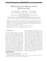
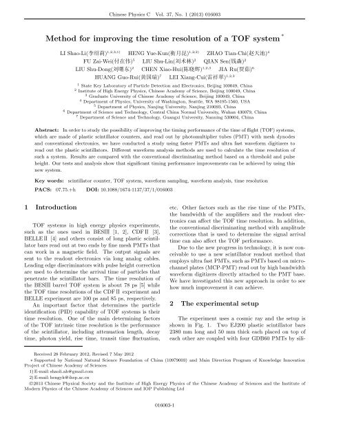
Chinese Physics C Vol. 37, No. 1 (2013) 016003Fig. 4. Diagram of calculating the start time, we only show part of the cosmic ray signal waveform so you can havea clear view: (a) the first method: simulating the traditional discriminating method; (b) the second method: linearfitting; (c) the third method: Landau fitting; and (d) the fourth method: fourth order polynomial fitting.Considering more points are used, the time value shouldbe more accurate than the first method.The third method (Fig. 4(c)) also uses data pointsinside an amplitude interval. The difference from thesecond method is that the interval is from 0% to 50% ofthe signal height and the model used is the Landau distribution.In Fig. 4(c), the Landau curve is drawn, whichcovers this interval and the time value can be obtainedbased on the Landau function and threshold value.The fourth method (Fig. 4(d)) uses data points insidean amplitude interval from 0% to 50% of the signalheight which is the same interval as we used in the thirdmethod. We try to use a polynomial curve fitting thedata points. Here we fit the data points with a fourthorder polynomial curve to obtain the discriminating timevalue.The time interval chosen in Method two is 20% to60% because the other part of the rising edge curves alot which does not fit the linear model. Since the morepoints you use in the third method the more fitting errorsyou will get [7], we choose the time interval from0% to 50% in Method three. This interval guaranteesthat enough waveform information will be used whilethe fitting error will not be too large. The fitting intervalchosen for method four is the same as with methodthree so we can compare results from these two differentfitting methods.The first method which calculates the time value onlyuses two points while the other three methods use moredata points from the waveform. We expect to see thatthe time resolution will be better if more waveform informationis used. Fig. 4 (b), (c) and (d) indicates thatthe Landau curve and polynomial curve fit the waveformbetter than the linear curve. This means the time resolutiongiven from Landau and polynomial fitting shouldbe better than the other two.Although the choice of fitting time interval can influencethe result, the third and fourth methods which usethe Landau and fourth order polynomial fitting give bettertime resolution than the other two methods. As westudied, changes in the time interval (like plus or minus10% of the signal amplitude) will not change the besttime resolution value much, but time resolution valuescalculated using a too small (like 5% or 10% of the signalamplitude) or big (like 40% of the signal amplitude)threshold value will vary a lot.3.4 Time resolution of the systemThere are four channels of signals from PMT GDB60and the discriminating time values are noted as T 1 , T 2 ,T 3 and T 4 . The time resolution of the system can becalculated based on this:T = (T 1+T 2 )−(T 3 +T 4 ), (5)4(T 1 +T 2 )−(T 3 +T 4 ) can reduce the hitting position variationof the cosmic ray and the uncertainty of start timeof the system.016003-4

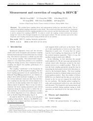
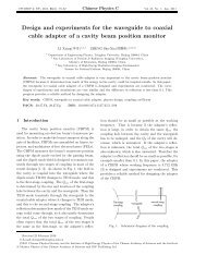
Chinese Physics C Vol. 37, No. 1 (2013) 016003Fig. 5. Time resolutions from four different methods for a threshold of 15% amplitude. All the events are takenfrom the same PMT. (a) the first method; (b) the second method; (c) the third method; (d) the fourth method.Figure 5 shows the examples of spectra of time Tcalculated from four different methods fitted by normaldistributions and the threshold value was assumed to be15% of the signal amplitude. The time resolution valuescalculated from the first, second, third and fourth methodsare 69.8 ps, 83.6 ps, 65.43 and 65.41 ps separately.The time resolution given from Fig. 5 is the time resolutionof one end. Our setup uses a two end readoutsystem, so the time resolution of one TOF counter hereis the value divided by √ 2. Fig. 6 shows the thresholdof different percentage vs. time resolution. Please notethat the time resolution values here have already beendivided by √ 2. The best time resolution of TOF readout at two ends is 46.3 ps using a Landau or polynomialfitting when the threshold is 15% of the signal amplitude.From Fig. 6, we can see that the Landau and polynomialfitting method give the best result while polynomialfitting is simpler. The linear fitting method is the worstone for the reasonable actual threshold value. In addition,the Landau curve fits the waveform better at thestarting part and worse at the crest part. The low thresholdarea corresponds to the starting area of the rise edgewhere the waveform curves a lot, that’s why the linearfitting become worse.Fig. 6. Threshold vs. time resolution with errorbars. TFM refers to the traditional fittingmethod. PFM refers to the linear fittingmethod. LFM refers to the Landau fittingmethod. POL4 refers to the fourth order polynomialfitting method.016003-5

Chinese Physics C Vol. 37, No. 1 (2013) 0160034 Conclusions and discussionsThe ultra fast PMT and waveform sampling techniqueused in our experiment significantly improve thetime resolution of the TOF system since detailed informationabout the signal shapes can be obtained from thewaveforms and used in the analysis.We have shown that among the four methods studied,the waveform analysis based on Landau and fourthorder polynomial curves are better than the traditionaldiscrimination method which give the best time resolutionof 46.3 ps, this is significantly better than the performanceof current TOF systems. This is due to the factthat more accurate information can be obtained by fittingthe rising edges of the recorded waveforms, which ismuch better than simply using a linear function extrapolation.Results from the first method are better thanwe have expected, mainly because the waveform informationis still used here to calculate the amplitude andthe start time. While the Landau, polynomial and linearfitting method rely on the choice of fitting time interval,the traditional fitting method only uses two recordedpoints.Technologies of a fast PMT and a high sampling ratewaveform digitizer are developing rapidly [8] and waveformdigitizers with 10 Gs/s sampling rate or higher maybecome available in the near future. They can be consideredto implement the techniques described in thispaper in the future TOF systems. The oscilloscope usedto record waveforms in our test would be replaced byintegrated high rate waveform digitizers that are compactand inexpensive. The long analog cables that limitsignal bandwidth in a conventional TOF system can beeliminated.References1 BES collaboration. Nucl. Instrum. Methods A, 2009, 598(1):72 BES Design Report, http://bes.ihep.ac.cn3 Paus Ch, Grozis C, Kephart R et al. Nucl. Instrum. MethodsA, 2001, 461(1–3): 5794 Kichimi H, Yoshimura Y, Browder T et al. Nucl. Instrum.Methods A, 2000, 453(1–2): 3155 HENG Yue-Kun. The Two Scintillator Detectors on BES.In: IEEE Nuclear Science Symposium and Medical ImagingConference. USA, NSS/MIC, 2007, (1): 536 WU Jing-Jie, HENG Yue-Kun, SUN Zhi-Jia et al. CPC (HEP& NP), 2008, 32(3): 1867 LIU Ji-Guo. Measurement Error Analysis and Time CorrectionMethod for Scintillator TOF Detector (Ph. D. Thesis). Hefei:University of Science and Technology of China, 20048 CAEN VX1761 Digitizer, http://www.caen.it/csite/CaenProd.jsp?showLicence=false&parent=1&idmod=673016003-6