Mixture Design Tutorial (Part 1 – The Basics) - Statease.info

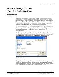
DX7-05A-Mix-P1.doc Rev. 3/14/06Mixture Design Tutorial(Part 1 – The Basics)IntroductionIn this tutorial you will get an introduction to mixture design. It will be assumed that atthis stage you’ve mastered many of Design-Expert® software’s basic features bycompleting the preceding tutorials. At the very least you ought to first do the GeneralOne-Factor tutorials, basic and advanced, prior to starting this one.We will presume that you can handle the statistical aspects of mixture design. To gain aworking knowledge of this powerful tool, we recommend you attend our Mixture Designfor Optimal Formulation workshop. Call Stat-Ease or visit our website,www.statease.com, for a schedule. If you want statistical detail on this topic, see, JohnCornell’s Experiments with Mixtures, 2nd edition published by John Wiley and Sons,New York in 1990.This tutorial provides only the essential program functions. For more details, check outthe Help system, which you can access at any time by pressing F1. Its hypertext searchcapability makes it easy for you to track down the information you need.The Case Study – Formulating a DetergentA detergent must be re-formulated to fine-tune two product attributes, which will bemeasured as responses from a designed experiment:• Y 1 - viscosity• Y 2 - turbidity.Three primary components will be varied as shown:• 3% ≤ A (water) ≤ 8%• 2% ≤ B (alcohol) ≤ 4%• 2% ≤ C (urea) ≤ 4%These components represent nine weight-percent of the total formulation, that is:A + B + C = 9%The other materials (held constant) make up the difference: 91 weight-percent of thedetergent. For purposes of this experiment they can be ignored.The experimenters chose a standard mixture design called a simplex-lattice. Theyaugmented this design with axial check blends and the overall centroid. The verticesDesign-Expert 7 User’s Guide Mixture Tutorial – Part 1 • 1

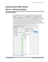
9070105050107090and overall centroid were replicated, which increased the size of the experiment to a totalof 14 blends.X 129070503023030102X 2X 3Augmented simplex lattice (second degree)2This case study leads you through all the steps of design and analysis for mixtures. Thenext tutorial, Part 2, will detail how you can simultaneously optimize the two responses.Design the ExperimentStart the program by finding and double clicking the Design-Expert software icon. Takethe quickest route to initiating a new design by clicking on the blank-sheet icon on theleft of the toolbar. The other route is via File, New Design (or associated Alt keys).Main menu and tool bar – New Design icon identifiedClick on the Mixture folder tab. The design you want, a simplex lattice, comes up bydefault.Choosing a mixture design2 • Mixture Tutorial – Part 1 Design-Expert 7 User’s Guide

High fields, pressing the Tab key after each entry. Enter 9 in the Total field and % inthe Units field.Entering components, limits and totalPress Continue. Immediately a warning appears.Adjustment made to constraintsPress OK. Notice that, although you entered the high limit for water as 8%,Design-Expert adjusts it to 5% which leaves room for 2% each of the other twoingredients within the 9% total. Otherwise, at 8% water and the low levels of alcoholand urea the total would become 12%, which the program realizes does not compute.Very smart and very helpful!Press Continue and this time the software lets you move on. Now you must choose theorder of the model that you expect to be appropriate for the system being studied. In thiscase, you can assume that a quadratic polynomial, which includes second order terms forcurvature, will adequately model the responses. Therefore leave the order atQuadratic. Accept the default check-off to Augment design, but change the Numberof runs to replicate to 3.Simplex-lattice design form (after pressing Tab key)By accepting “Augment design” you allow Design-Expert to add the overall centroidand axial check blends to the design points. The “Number of runs to replicate” field,4 • Mixture Tutorial – Part 1 Design-Expert 7 User’s Guide

DX7-05A-Mix-P1.doc Rev. 3/14/06defaulted to 4, causes the specified number of highest leverage experiments to beduplicated. In this case, there are three points with highest leverage – the vertices of thetriangular simplex.Press Continue to the next step in the design process: Entering Responses. For thenumber select 2. Then enter the response Names and Units as shown below.Response entryYou can step Back through the design forms and change what you want anywhere alongthe way. When you press Continue on this page, Design-Expert will complete thedesign setup for you.Examine the Design and Modify It If You LikeRight click on the top of the Block column in the design layout and select DisplayPoint Type. (The program randomizes run order, so do not worry about standard(“Std”) order differing on your screen from what’s shown here.)Displaying point type (Your Std order numbers vary due to randomization)Then right click the top of the column labeled Std and select Display Design ID.Displaying design IDDesign-Expert 7 User’s Guide Mixture Tutorial – Part 1 • 5

Again, right click the top of the column now labeled Id, but this time select Sort byDesign ID. Now you get a feel for where the points are located and which ones arereplicated. (Run order is randomized and thus differs from what’s shown below.)Initial design sorted by ID with point type shown (run order randomized)The experimenters ran an additional centroid point, so in the box to the left of Id 0(Type: “Center”) right-click and select Duplicate.Duplicating the centroidWhenever you insert, delete or duplicate rows, always right-click the Run columnheaderand chose Randomize.Re-randomizing the run orderA box will pop up asking if you’d like all blocks to be randomized. In this case there isonly one block, so simply press OK. Notice that run numbers now change.6 • Mixture Tutorial – Part 1 Design-Expert 7 User’s Guide

DX7-05A-Mix-P1.doc Rev. 3/14/06Again, right-click the Run column-header, but this time choose Sort by Run Order.Normally you’d now do a File, Print to produce a ‘recipe’ sheet for doing theexperiment. Go ahead if you have a printer available.Save Your WorkAnalyze the ResultsNow that you’ve invested some time into your design, it would be prudent to save yourwork. Click on File menu item and select Save As. The program displays a standardfile dialog box. Use it to specify the name and destination of your data file. Enter a filename in the field with the default extension of dx7. (We suggest tut-mix). Then clickon Save.Assume that the experiments are now complete. You now need to enter the responsesinto the Design-Expert software. For tutorial purposes, we see no benefit to making youtype all the numbers. Therefore, to save time, read the response data in from a file thatwe’ve put on your program’s Data directory. Select File, Open Design. Click on thefile called Mix.dx7. Then press OK. You now should see response data.There’s no need for typing in this case, but normally you’d have put in a lot more workat this stage, so always do a File, Save for preservation of entered response data.Response dataGo to the Analysis branch of Design-Expert and click on the node for Viscosity. Younow will work across the buttons at the top of the window.Design-Expert 7 User’s Guide Mixture Tutorial – Part 1 • 7

First step in analysis: Transformation optionsFirst, consider doing a transformation on the response. In some cases this will improvethe statistical properties of the analysis. For example, when responses vary over severalorders of magnitude, the log scale usually works best. In this case the ratio of maximumto minimum response is only a bit over 4, which isn’t too excessive (see detail at bottomof the screen), so leave the selection at its default, None, because no transformation willbe needed. Also, leave the coding for analysis as pseudo which re-scales the actualcomponent levels to 0 – 1. For complete details on coding mixtures see the textbook byCornell mentioned at the outset of the tutorial. In the meantime, bring up Help,Contents and then double-click Mixture Designs and Mixture StatisticalInformation and then select Component Scaling in Mixture Designs.Statistical detail on coding available via HelpClose Help down by pressing X. Then click on the Fit Summary button. At this pointDesign-Expert fits linear, quadratic, special cubic and full cubic polynomials to theresponse.8 • Mixture Tutorial – Part 1 Design-Expert 7 User’s Guide

DX7-05A-Mix-P1.doc Rev. 3/14/06Fit summary reportsYou may need to widen your window to get the entire output showing. Just move thecursor to the left edge until it changes to a double-ended arrow. Then drag it open. Insimilar fashion, you can also adjust column widths in any table or report. This may benecessary to uncover the entire text. To move around the display, use the side and/orbottom scroll bars, if necessary.First, look for any warnings about aliasing. In this case, the full cubic model could notbe estimated by the chosen design – an augmented simplex design. Remember that youchose only to fit a quadratic model, so this should be no surprise.Next, you see the “Sequential Model Sum of Squares” table. The analysis proceedsfrom a basis of the mean response. This is the default model if none of the factors causea significant effect on the response. The output then shows the significance of each setof additional terms:• “Linear vs Mean”: the significance of adding the linear terms afteraccounting for the mean. (Due to the constraint that the three componentsmust sum to a fixed total, you will see only two degrees of freedomassociated with the linear mixture model.)• “Quadratic vs Linear”: the significance of adding the quadratic terms to thelinear terms already in the model.• “Sp Cubic vs Quadratic”: the contribution of the special cubic terms beyondthe quadratic and linear terms.• “Cubic vs Sp Cubic”: the contribution of the full cubic terms beyond thespecial cubic, quadratic, and linear terms. (In this case, these terms arealiased.)Design-Expert 7 User’s Guide Mixture Tutorial – Part 1 • 9

For each set of terms, the probability (“Prob > F”) should be examined to see if it fallsbelow 0.05 (or whatever statistical significance level you choose). Adding terms up toquadratic will significantly improve this particular model, but when you get to thespecial cubic level, there’s no further improvement. The program automaticallyunderlines at least one “Suggested” model. Always confirm this suggestion byreviewing all the tables under Fit Summary.The lack of fit table compares the residual error to the pure error from replication. If theresidual error significantly exceeds the pure error, then something remains in theresiduals that can be removed by a more appropriate model. The residual error from thelinear model shows significant lack of fit (bad), while the quadratic, special cubic andfull cubic do not show significant lack of fit (good). At this point the quadratic modellooks very good.Lack of fit tableNow, scroll down to the last table: “Model Summary Statistics.” Here you see severalcomparative measures for model selection.Summary statisticsIgnoring the aliased cubic model, the quadratic model comes out best: low standarddeviation (“Std Dev”), high “R-Squared” statistics and low “PRESS.”Before moving on, you may want to print the Fit Summary tables by doing a File, Print.These tables, or any selected subset, can be also cut and pasted into a word processor,spreadsheet or any other Window’s application. You’re now ready to take an in-depthlook at the quadratic model.10 • Mixture Tutorial – Part 1 Design-Expert 7 User’s Guide

DX7-05A-Mix-P1.doc Rev. 3/14/06Model Selection and Analysis of Variance (ANOVA)Click the Model button to see the model suggested by Design-Expert software. Pressthe screen tips button to see some very helpful information about what you can do atthis stage.Choosing the model (Tips up on screen)You may select alternate models to the default, in this case quadratic, from the pull downlist if you want. (Be sure to do this in the rare cases when Design-Expert suggests morethan one model.) On this screen you are allowed to manually reduce the model byclicking off terms that are not statistically significant. For example, in this case, you willsee in a moment that the AB term is not statistically significant.As noted under the heading “Model Reduction” in Tips, Design-Expert provides severalautomatic reduction algorithms as alternatives to the manual method: Backward,Forward and Stepwise. Click the down arrow on the list box if you’d like to try one.We recommend that you not reduce mixture models unless you’re sure from subjectmatter knowledge that this makes sense.Close Tips by clicking X. The press the ANOVA button for the details on the quadraticmodel. There are two views available for the ANOVA report: plain or annotated. Fortutorial purposes it’s best you keep it in View, Annotated ANOVA to help with theinterpretation. The program will default to whichever view was last chosen.Design-Expert 7 User’s Guide Mixture Tutorial – Part 1 • 11

ANOVA report with annotations toggled onThe statistics look very good. The model has a high F value, low probability values(Prob > F). The probability values show the significance of each term. Because themixture model does not contain an intercept term, the main effect coefficients (linearterms) incorporate the overall average response and are tested together. Scroll down tothe next report with R-squared statistics.R-squared and other statistics after the ANOVAThese statistics, many of these you’ve seen already in the “Model Summary Statistics”table, all look good. Note the more than adequate precision value of 27.9.12 • Mixture Tutorial – Part 1 Design-Expert 7 User’s Guide

DX7-05A-Mix-P1.doc Rev. 3/14/06Scroll down and take a look at the coefficients and associated confidence intervals forthe quadratic model.Coefficients for the quadratic modelContinue on to see several alternative models that vary by how the components arecoded. This may be of most interest to students of mixture design rather than actualformulators, so it’s time to move on: Press the next button – Diagnostics.Diagnose the Statistical Properties of the ModelThe most important diagnostic, the normal probability plot of the residuals, comes up bydefault.Normal Probability Plot of the ResidualsThe data points should be approximately linear. A non-linear pattern (look for an S-shaped curve) indicates non-normality in the error term, which may be corrected by atransformation. There are no signs of any problems in our data.Design-Expert 7 User’s Guide Mixture Tutorial – Part 1 • 13

At the left of the screen you see the Diagnostics Tool palette. First of all, notice thatresiduals will be studentized unless you uncheck the first box on the floating tool palette(not advised). This counteracts varying leverages due to location of design points. Forexample, the center points carry little weight in the fit and thus exhibit low leverage.Each button on the palette represents a different diagnostics graph. Check out the othergraphs if you like. Explanations for most of these graphs were covered in priorTutorials. In this case, none of the graphs indicate any cause for alarm.Now click the option for Influence. Here’s where you find the find plots for externallystudentized residuals (better known as “outlier t”) and other plots that may be helpful forfinding problem points in the design. Also, from here you can bring up case-by-casedetails on many of the statistics shown graphically for diagnostic purposes: PressReport. (In previous versions of Design-Expert, this report appeared under ANOVA.)Diagnostics reportNotice that one value is flagged for exceeding suggested limits: DFFITs for standardorder 11. As we discussed in the General One-Factor Tutorial (Part 2 – AdvancedFeatures), this statistic stands for difference in fits. It measures the change in eachpredicted value that occurs when that response is deleted. Given that only this onediagnostic is flagged, it probably is not a cause for alarm. However, observe that it’s thehighest observed viscosity response (130.00 Actual Value) , so the experimenter oughtto double-check the accuracy of this response.Examine Model GraphsThe diagnosis of residuals reveals no statistical problems, so you will now generate theresponse surface plots. Click on the Model Graphs button. The 2D contour plot ofcomes up by default in graduated color shading.14 • Mixture Tutorial – Part 1 Design-Expert 7 User’s Guide

DX7-05A-Mix-P1.doc Rev. 3/14/06Response surface contour plotNote that Design-Expert will display any actual point included in the design spaceshown. In this case you see a plot of conversion as a function of time and temperature ata mid-level slice of catalyst. This slice includes two centroids as indicated by the dot atthe middle of the contour plot.The Factors Tool comes along with the default plot. Move this floating tool as neededby clicking on the top blue border and dragging it. The tool controls which factor(s) areplotted on the graph. The Gauges view is the default. Each component listed will eitherhave an axis label, indicating that it is currently shown on the graph, or a red slider bar,which allows you to choose specific settings for those not currently plotted. This casestudy involves only three components, all of which can fit on one mixture plot – aternary diagram. Therefore, you will not see a slider bar. If you did, it would default tothe midpoint levels of the components not currently assigned to axes. You could thenchange a level by dragging the red slider bars. If you’d like to see a demonstration ofthis feature, do the Multifactor RSM Tutorial (Part 1 – The Basics).Place your mouse cursor over the contour graph. Notice in the lower left corner of thescreen that Design-Expert displays the predicted response and coordinates.Coordinates display at lower, left corner of screenDesign-Expert 7 User’s Guide Mixture Tutorial – Part 1 • 15

To enable a handier tool for reading coordinates off contour plots, go to View, ShowCrosshairs Window.Showing crosshairs windowNow move your mouse over the contour plot and notice that Design-Expert generatesthe predicted response for specific values of the factors that correspond to that point. Ifyou place the crosshair over an actual point, for example – the check-blend above thecentroid, you also get that observed value (in this case: 35.1).Zooming In and OutPrediction at upper check blend where an actual run was performed (Small vs Full)Press the Full button to get confidence and prediction intervals in addition to thecoordinates and predicted response. Then close out the crosshairs window by clickingX.Let’s say you were particularly interested in highest values for viscosity. With your leftmouse button pressed, drag over an empty area on the graph over to the left as shownbelow.16 • Mixture Tutorial – Part 1 Design-Expert 7 User’s Guide

DX7-05A-Mix-P1.doc Rev. 3/14/06Creating a designated area by dragging the mouseIf your graph disappears entirely and you get the message “Can’t create contour graph”,press the Default button the Factors Tool. Now drag over the lower right corner of thecontour graph.Corner identified for zoomNow you see just the area you chose magnified.Zoomed-in area on contour plotDesign-Expert 7 User’s Guide Mixture Tutorial – Part 1 • 17

To revert back to the full triangle, right-click over the plot and select Zoom out.Zoom outTrace PlotWouldn’t it be handy to see all your factors on one response plot? You can do this withthe trace plot, which provides silhouette views of the response surface. The real benefitfrom this plot is for selecting axes and constants in contour and 3D plots. Use the View,Trace menu item to select it.Trace plot – component A highlightedThe trace plot shows the effects of changing each component along an imaginary linefrom the reference blend (defaulted to the overall centroid) to the vertex. As the amountof this component increases, the amounts of all other components decrease, but theirratio to one another remains constant. Click on the curve for A. (It will change color).Notice that viscosity is not very sensitive to this component.The floating Trace Graph menu offers various options for the directions taken by thetraces and the method. In this case where the experimental region forms a simplex, itmatters little which choices you make. See for yourself by pressing the alternatives towhat’s provided by default.18 • Mixture Tutorial – Part 1 Design-Expert 7 User’s Guide

DX7-05A-Mix-P1.doc Rev. 3/14/06Contour Plot: RevisitedIf you experiment on more than three mixture components, use the trace plot to findthose components that most affect the response. Choose these influential componentsfor the axes on the contour plots. Set as constants those components that createrelatively small effects. Your 2D contour and 3D plots will then be sliced up in waythat’s most interesting visually.Return to the contour plots via the View, Contour selection. The colors are neat, butwhat if you must print the graphs in black and white? That can be easily fixed by rightclickingover the graph and selecting Graph Preferences. Then click the Graphs 2tab and change the Contour graph shading to Std Error shading.Graph preferences: Changing contour graph shadingPress OK to see the effect on your plot.Contour plot with standard error shadingDesign-Expert draws five contour levels by default. They range from the minimumresponse to the maximum response. Click on a contour to highlight it. You can movethe contours by dragging them to new values. (Place the mouse cursor on the contourand hold down the left button while moving the mouse.) Give this a try – it’s fun!Design-Expert 7 User’s Guide Mixture Tutorial – Part 1 • 19

We recommend another approach to laying out contours. Right click in the drawing orlabel area of the graph and choose Graph Preferences. Then choose Contours.Now select the Incremental option and fill in the Start at 35, Step at 10 and Levelsat 20. Also, under Format choose 0 to display whole numbers (no decimals). Yourscreen should now match that shown below.Contours dialog box: Incremental optionPress OK to get a good-looking contour plot – suitable for printing. This one wasproduced via Edit, Copy from Design-Expert and Edit, Paste into Microsoft Word. (Thetriangle may not come in looking equilateral, but if this is bothersome, it can be easilyremedied by dragging the right border and widening the picture.)Plot with incremental contours20 • Mixture Tutorial – Part 1 Design-Expert 7 User’s Guide

DX7-05A-Mix-P1.doc Rev. 3/14/06You can add new contours via a right mouse click. Find a vacant region on the plot, forexample – between the 35 and 45 contours, and check it out: Right-click and select Addcontour. Then drag the contour around (it will become highlighted) until it becomes40.Adding contoursTo get a more precise contour level and locate it accurately, you can right-click it andenter the desired value. Try this on the new contour labeled 40.Setting a contour valueThat fills a gap nicely!Move your mouse to a spot near the top of the graph, where the response hits theminimum. Click the right mouse button and Add flag. To get more digits displayed,right click for Graph Preferences and under Contours change Format to 0.00.Then press OK.Adding a flag (format re-set via Graph Preferences)It displays the value of the response at that point. Now do a right click of the mouse onthe flag and select Toggle size.Design-Expert 7 User’s Guide Mixture Tutorial – Part 1 • 21

Flag enlarged via Toggle Size optionThe expanded flag displays a 95 percent confidence interval (CI) on the mean prediction.It also provides the prediction interval (PI). Use this to ‘manage expectations’ aboutindividual confirmation runs near this point. The PI conveys how natural variability inthe process/sampling/testing plus imprecision in the estimate of the mean (SE mean)causes actual outcomes to differ from the prediction. The larger flag also lists the pointcoordinates. If you have a printer, you can print the contour plot by using the File, Printmenu item.Generating a 3D View of the Response SurfaceNow to really get a feel for how the response varies as a function of the two factorschosen for display, select View, 3D Surface. You then will see three-dimensionaldisplay of the response surface. If the coordinates encompass actual design points, thesewill be displayed.3D response surface plotThe Rotation tool allows you to view the 3D surface plot from any angle.22 • Mixture Tutorial – Part 1 Design-Expert 7 User’s Guide

DX7-05A-Mix-P1.doc Rev. 3/14/06Control for rotating 3D plotMove your cursor over the tool. The pointer changes to a hand. Now use the hand torotate the vertical or horizontal wheel. Watch the 3D surface change. It’s fun! What’sreally neat is how it becomes transparent so you can see hidden points falling below thesurface.Response PredictionTransparent view as surface is rotated, which allows points to be seen betterAlso, be aware that Design-Expert offers many options for 3D graphs via its preferences,which come up via a right-click over the plot. For example, if you don’t like thegraduated colors, go to the Graphs 2 tab and change the 3D graph to the hidden wireview (a transparent look).Press the Default button when you’re done playing. The graph then re-sets to its originalposition. Notice that you can also specify the horizontal (“h”) and vertical (“v”)coordinates.This feature in Design-Expert software falls under the Optimization branch, which willbe explored more fully in the next tutorial in this series. It allows you to generatepredicted response(s) for any set of factors. To see how this works, click on the PointPrediction node (lower left on your screen).Design-Expert 7 User’s Guide Mixture Tutorial – Part 1 • 23

Point PredictionYou now see the predicted responses from this particular blend - the centroid. Be sure tolook at the 95% prediction interval (“PI low” to “PI high”). This tells you what toexpect for an individual confirmation test. You might be surprised at how muchvariability could affect the outcome. You can print the results by using the File, Printcommand.The Factors Tool will open along with the point prediction window. Move thefloating tool as needed by clicking on the top border and dragging it. You can drag thehandy sliders on the component gauges to look at other blends. Note that in a mixtureyou can only vary two of the three components independently. Can you find acombination that produces viscosity of 43? (Hint: push Urea up a bit.) Don’t try toohard, because in the next section of this tutorial you will make use of Design-Expert’soptimization features to accomplish this objective.Click on the Sheet button to get a convenient entry form for specific component values.Be careful though, the ingredients must add up to the fixed total you specified – in thiscase 9 wt %. Design-Expert will make adjustments as you go – perhaps in ways that youdo not anticipate. Don’t worry: If you get too far off, simply press the Default button toget back to the centroid.Analyze the Data for the Second ResponseThe last step is a BIG one. Analyze the data for the second response, turbidity (Y 2 ). Besure you find the appropriate polynomial to fit the data, examine the residuals and plotthe response surface. (Hint: The correct model is special cubic.)Before you quit, do a File, Save to preserve your analysis. Design-Expert will saveyour models. To leave Design-Expert, use the File, Exit menu selection. The programwill warn you to save again if you’ve modified any files.This tutorial gets you off to a good start using Design-Expert software for mixtures. Wesuggest that you now go on to the Mixture Optimization Tutorial. You also may want todo the tutorials on use of response surface methods (RSM) for process variables. Tolearn more about mixture design, attend Mixture Design for Optimal Formulation, athree-day workshop presented by Stat-Ease. Call or visit our web site(www.statease.com) for a schedule.24 • Mixture Tutorial – Part 1 Design-Expert 7 User’s Guide