Mixture Design Tutorial (Part 2 – Optimization) - Statease.info

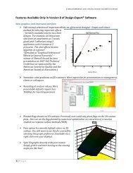
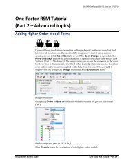
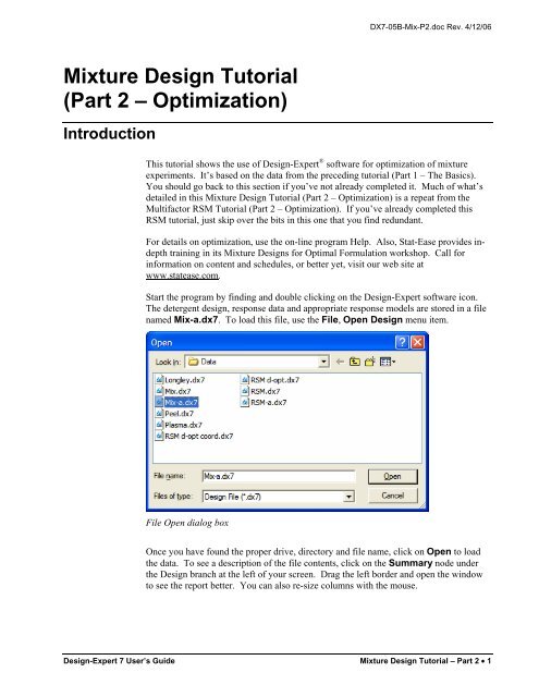
DX7-05B-Mix-P2.doc Rev. 4/12/06Mixture Design Tutorial(Part 2 – Optimization)IntroductionThis tutorial shows the use of Design-Expert ® software for optimization of mixtureexperiments. It’s based on the data from the preceding tutorial (Part 1 – The Basics).You should go back to this section if you’ve not already completed it. Much of what’sdetailed in this Mixture Design Tutorial (Part 2 – Optimization) is a repeat from theMultifactor RSM Tutorial (Part 2 – Optimization). If you’ve already completed thisRSM tutorial, just skip over the bits in this one that you find redundant.For details on optimization, use the on-line program Help. Also, Stat-Ease provides indepthtraining in its Mixture Designs for Optimal Formulation workshop. Call forinformation on content and schedules, or better yet, visit our web site atwww.statease.com.Start the program by finding and double clicking on the Design-Expert software icon.The detergent design, response data and appropriate response models are stored in a filenamed Mix-a.dx7. To load this file, use the File, Open Design menu item.File Open dialog boxOnce you have found the proper drive, directory and file name, click on Open to loadthe data. To see a description of the file contents, click on the Summary node underthe Design branch at the left of your screen. Drag the left border and open the windowto see the report better. You can also re-size columns with the mouse.Design-Expert 7 User’s Guide Mixture Design Tutorial – Part 2 • 1

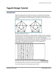
DX7-05B-Mix-P2.doc Rev. 4/12/06Setting the Optimization CriteriaDesign-Expert allows you to set criteria for all variables, including components andpropagation of error (POE). (We will get to POE later.) The limits for the responsesdefault to the observed extremes.Now you get to the crucial phase of numerical optimization: assignment of“Optimization Parameters.” The program uses five possibilities for a “Goal” toconstruct desirability indices (d i ):• Maximize,• Minimize,• Target->,• In range,• Equal to -> (components only).Desirabilities range from zero to one for any given response. The program combines theindividual desirabilities into a single number and then searches for the greatest overalldesirability. A value of one represents the ideal case. A zero indicates that one or moreresponses fall outside desirable limits. Design-Expert uses an optimization methoddeveloped by Derringer and Suich, described by Myers and Montgomery in ResponseSurface Methodology, John Wiley and Sons, New York (available from Stat-Ease).In this case the components will be allowed to range within their pre-establishedconstraints, but be aware that they can be set to desired goals. For example, since wateris cheap, you could set its goal to maximize.Options for goals on componentsNotice that components can be set equal to a specified level. Leave water at its defaultof “in range” and click the first response Viscosity. Set its Goal at target-> of 43.Enter Limits at Lower of 39 and Upper of 48.Design-Expert 7 User’s Guide Mixture Design Tutorial – Part 2 • 3

Setting Target for first response of viscosityThese limits indicate that it is most desirable to achieve the targeted value of 43, butvalues in the range of 39-48 are acceptable. Values outside that range have no (zero)desirability.Now click on the second response, Turbidity. Select the Goal of minimize, withLimits set at Lower of 800 and Upper of 900. You must provide both thesethresholds to get the desirability equation to work properly. By default they will be setat the observed response range, in this case 321 to 1122. However, evidently in this casethere’s no advantage to getting the detergent’s turbidity below 800 – it already appearsas clear as can be to the consumer’s eye. On the other hand, when turbidity exceeds 900,it looks as bad as it gets.Aiming for minimum on second response of turbidity4 • Mixture Design Tutorial – Part 2 Design-Expert 7 User’s Guide

Weights change by grabbing handle with mouseNotice that the Weight now reads 10. You’ve now made it much more desirable to getnear the goal of 800 for turbidity. Before moving on from here, re-enter the UpperWeights at its default value of 1. This will straighten out to the desirability ramp.“Importance” is a tool for changing the relative priorities for achieving the goals youestablish for some or all of the variables. If you want to emphasize one over the rest, setits importance higher. Design-Expert offers five levels of importance ranging from 1plus (+) to 5 plus (+++++). For this study, leave the Importance field at +++, amedium setting. By leaving all importance criteria at their default, none of the goals willbe favored over any other.For an in-depth explanation of the construction of the desirability function, and formulasfor the weights and importance, select Help off the main menu. Then go to Contentsand select Optimization. Branch down to the topic of Importance as shown on thescreen-shot below. From there you can open various topics and look for the details youneed.Details on Importance found in program Help6 • Mixture Design Tutorial – Part 2 Design-Expert 7 User’s Guide

DX7-05B-Mix-P2.doc Rev. 4/12/06When you are done looking at Help, close out the screen by pressing X at the upper-rightcorner of its screen.Click the Options button to see how you gain control over how the numericaloptimization will be performed. For example, you can change the number of cycles(searches) per optimization. If you have a very complex combination of responsesurfaces, increasing the number of cycles will give you more opportunities to find theoptimal solution. The Duplicate solution filter establishes the epsilon (minimumdifference) for eliminating essentially identical solutions. The Simplex Fractionspecifies how big the initial steps will be relative to the factor ranges. (The word“simplex” relates to the geometry of the search. For two factors the simplex is anequilateral triangle. By stepping through the three corners the program figures out thepath of steepest ascent. For more detail, go to Help and search on “numerical searchalgorithm.”)Another optimization option is to not use random starting points, but rather those in thedesign itself. However, these will be limited to 100 unless you change this default.Leave this and all other options at their default levels shown below. (PS. This screenshot shows underlined letters that show Alt keys for jumping to fields via keystrokesversus mousing.)Optimization Options Dialog BoxRunning the optimizationStart the optimization by clicking on the Solutions icon.Design-Expert 7 User’s Guide Mixture Design Tutorial – Part 2 • 7

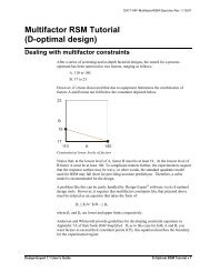
DX7-05B-Mix-P2.doc Rev. 4/12/06The ramp display combines the individual graphs for easier interpretation. The dot oneach ramp reflects the factor setting or response prediction for that solution. The heightof the dot shows how desirable it is. Press the different solution buttons (1, 2, 3,…) andwatch the dots. The red ones representing the component levels move around quite a bit,but do the responses remain within their goals (desirability of 1)? Click the last solutionon your screen. Does it look something like the one below?Sub-optimum solution that ranks least desirableIf your search also uncovered this local optimum, you will note that viscosity falls offtarget and turbidity becomes excessive, thus making it less desirable than the option forhigher temperature.Select the Bar Graph view.Solution to multiple response optimization - desirability bar graphDesign-Expert 7 User’s Guide Mixture Design Tutorial – Part 2 • 9

Finally, to make the graph really plain, go to the Fonts & Colors tab, choose ContourBackground, click Edit Color and select white off the grid and press OK.Graph changed to black and white with grid linesThere are many other options on this and other tabs for Graph preferences. Look themover if you like and then press OK to see what the options specified by this tutorial dofor your contour plot. If you like, look at the optimal turbidity response as well.To look at the desirability surface in three dimensions, click again on Response andchoose Desirability. Then select View, 3D Surface from the main menu.3D view of desirability at default resolution in colorIn this case the desirability surface is a bit too jaggedy for the colors to provide muchadvantage for interpretation, so right-click over the graph and select GraphPreferences. On the Graphs 1 tab change the Graph resolution to High. ThenOn the Graphs 2 tab change the 3D graph drawing method to Std errorshading.12 • Mixture Design Tutorial – Part 2 Design-Expert 7 User’s Guide

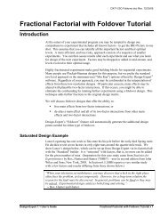
DX7-05B-Mix-P2.doc Rev. 4/12/06Changing graph preferences for the 3D plotPress OK for the new graph preferences. Then to get the view shown below, go to theRotation tool and change the horizontal control h to 350 and v to 85. Click on thegraph for a spectacular view!Shaded 3D desirability plot at high resolutionNow you can see two high ridges where desirability can be maintained at a maximumlevel over a range of compositions. The other peak is less desirable.When you have more than three components to plot, Design-Expert software uses thecomposition at the optimum as the default for the remaining constant axes. For example,if you design for four components, the experimental space is a tetrahedron. Within thisthree-dimensional space you may find several optimums, which require multipletriangular “slices,” one for each optimum.The best way for pointing out the most desirable formulation for your mixture is todemonstrate it on your computer screen or with the output projected for a largeraudience. In this case, you’d best shift back to the default colors and other displayschemes. Do this by right-clicking and selecting Graph Preferences and pressing theDefault buttons for the Graphs 1, Graphs 2 and Fonts and Colors (Colors sideonly).Design-Expert 7 User’s Guide Mixture Design Tutorial – Part 2 • 13

DX7-05B-Mix-P2.doc Rev. 4/12/06The surface reaches a minimum where the least amount of error is transmitted, orpropagated, to the viscosity response. These minima occur at the flat regions on themodel graphs where formulations will be most robust to varying amounts ofcomponents.Click on the Turbidity node, press the Model Graphs button and select View,Propagation of Error and look at its 3D Surface. Rotate it so you can see thesurface best.POE surface for turbidityFor additional details on POE, attend Stat-Ease’s Robust Design, DOE Tools forReducing Variability workshop.Now that you’ve found optimum conditions for the two responses, let’s go back and addcriteria for the propagation of error. Click on the Numerical optimization node. Selectthe POE (Viscosity) and establish a Goal to minimize with Limits of Lower at 5and Upper of 8.Set goal and limits for POE (Viscosity)Design-Expert 7 User’s Guide Mixture Design Tutorial – Part 2 • 15

DX7-05B-Mix-P2.doc Rev. 4/12/06Viewing Trace Plots from Optimal PointPress ahead to the numerical optimization Graphs to look at the contour plot fordesirability. It will not look much different that before, because adding criteria on POEhad only a small impact on the result. However, this will be a good time to get a feel forthe sensitivity of responses around the optimum point. See this by changing theChanging the response to be viewed from the optimum pointThen select View, Trace and click solutions 2 and beyond to see how it shifts withvarying optimal reference points. Return to Solution 1, which may produce the tracepictured below (remember that your results may vary due to random elements in thenumerical search algorithm employed by Design-Expert software).Trace plot viewed from optimal pointTake a look at the trace for the other response – turbidity. It looks even moreinteresting!Design-Expert 7 User’s Guide Mixture Design Tutorial – Part 2 • 17

Setting the turbidity contour valuePress OK to get the cleaner contour level. Right-click over the flag and select Deleteflag to make it easier to see how this change in turbidity affects the sweet spots. Noticethat the smaller one has now disappeared.Changing the specification on turbidity to 750 maximumGraphical optimization works great for three components, but as the number increases, itbecomes more and more tedious. You will find solutions much more quickly by usingthe numerical optimization feature. Then return to the graphical optimization andproduce outputs for presentation purposes.Response Prediction at the OptimumClick on the Point Prediction node (lower left on your screen). Notice how it nowdefaults to the first solution.20 • Mixture Design Tutorial – Part 2 Design-Expert 7 User’s Guide

DX7-05B-Mix-P2.doc Rev. 4/12/06Point prediction set to solution #1Save the Data to a FileNow that you’ve invested all this time into setting up the optimization for this design, itwould be prudent to save your work. Click on the File menu item and select Save As.Save As selectionFinal CommentsYou can then specify the File name (we suggest tut-MIX-opt) to Save as type *.dx7”in the Data folder for Design-Expert (or wherever you want to Save in).We feel that numerical optimization provides powerful insights when combined withgraphical analysis. Numerical optimization becomes essential when you investigatemany components with many responses. However, computerized optimization will notwork very well in the absence of subject matter knowledge. For example, a naive usermay define impossible optimization criteria. The result will be zero desirabilityeverywhere! To avoid this, try setting broad acceptable ranges. Narrow them down asyou gain knowledge about how changing factor levels affect the responses. Often, youwill need to make more than one pass to find the “best” factor levels to satisfyconstraints on several responses simultaneously.With Design-Expert software, you can explore the impact of changing multiplecomponents on multiple responses, and find maximally desirable solutions quickly vianumerical optimization. (Don’t forget that you can set goals on the componentsthemselves – for example, in this case it might be wise to try maximizing the amount ofcheap water.) For your final report, finish up with a graphical overlay plot at theoptimum “slice.”Design-Expert 7 User’s Guide Mixture Design Tutorial – Part 2 • 21

Learn more about methods of mixture design at our Mixture Designs For OptimalFormulation workshop. To get the latest class schedules, give Stat-Ease a call. Also, weappreciate your questions and comments on Design-Expert software. Call us, send anannotated fax of output, write us a letter or send us an e-mail. You will find our contactinformation and email links at www.statease.com.22 • Mixture Design Tutorial – Part 2 Design-Expert 7 User’s Guide