sercdp0172

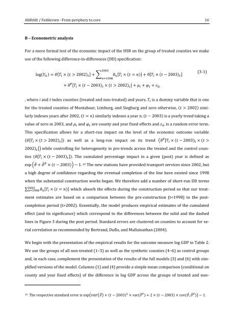
Ahlfeldt / Feddersen –From periphery to core 16B – Econometric analysisFor a more formal test of the economic impact of the HSR on the group of treated counties we makeuse of the following difference-in-differences (DD) specification:log(Y it ) = θ[T i × (t > 2002) t ] + ∑2002n=1998θ n [T i × (t = n)] + ϑ[T i × (t − 2003) t ](3-1)+ ϑ P [T i × (t − 2003) t × (t > 2002) t ] + μ i + φ t + ε it, where i and t index counties (treated and non-treated) and years, T i is a dummy variable that is onefor the treated counties of Montabaur, Limburg, and Siegburg and zero otherwise, (t > 2002) similarlyindexes years after 2002, (t = n) similarly indexes a year n, (t − 2003) is a yearly trend taking avalue of zero in 2003, and μ i and φ t are county and year fixed effects and ε it is a random error term.This specification allows for a short-run impact on the level of the economic outcome variable(θ[T i × (t > 2002) t ]) as well as a long-run impact on its trend (ϑ P [T i × (t − 2003) t × (t >2002) t ]) while controlling for heterogeneity in pre-trends across the treated and the control counties(ϑ[T i × (t − 2003) t ]). The cumulated percentage impact in a given (post) year is defined asexp (θ̂ + θ̂ P × (t − 2003)) − 1. 10 The new stations have provided transport services since 2002, buta high degree of confidence regarding the eventual completion of the line have existed since 1998when the substantial construction works began. We therefore add a number of short-run DD terms2002∑n=1998 θ n [T i × (t = n)] which absorb the effects during the construction period so that our treatmentestimates are based on a comparison between the pre-construction (t2002). Essentially, the model produces empirical estimates of the cumulatedeffect (and its significance) which correspond to the differences between the solid and the dashedlines in Figure 3 during the post period. Standard errors are clustered on counties to account for serialcorrelation as recommended by Bertrand, Duflo, and Mullainathan (2004).We begin with the presentation of the empirical results for the outcome measure log GDP in Table 2.We use the groups of all non-treated (1–3) as well as the synthetic counties (4–6) as control groupsand, in each case, complement the presentation of the results of the full models (3) and (6) with simplifiedversions of the model. Columns (1) and (4) provide a simple mean comparison (conditional oncounty and year fixed effects) of the difference in log GDP across the groups of treated and non-10 The respective standard error is exp(var(θ̂) + (t − 2003) 2 × var(θ̂ P ) + 2 × (t − 2003) × cov(θ̂, θ̂ P )) − 1.