sercdp0172

Recommendations

Info

Ahlfeldt / Feddersen –From periphery to core 27points with the estimated market potential elasticity the predicted increase in GDP for Montabaur isabout 6%, which is close to the cumulated effect after three years detected in the program evaluationsection.The remaining columns in Table 5 present results according to Eq. (4-3) replacing regional GDP withthe GVA of various industry sectors as the outcome variable. The estimated spillover effects are visualizedin Figure 5 as gray lines. The estimates are generally within the range of column (1). For somesectors the parameters are, however, estimated less precisely. The results also suggest that the marketpotential elasticity estimated in column (1) is brought down somewhat by sectors that are apparentlyless susceptible to agglomeration benefits, namely services other than financial services. Forconstruction, mining, manufacturing, and financial services the elasticity of output with respect tomarket potential is relatively large.As the HSR line is used exclusively for passenger transport, we expect to capture Marshallian externalitiesrelated to human interactions. Candidates are knowledge spillovers due to formal and informalmeetings, improved labor market access and matching, as well as improved access to intermediatedgoods and consumer markets to the extent that the ease of communication reduces transactioncosts but not freight costs. Our results are thus principally comparable to Ahlfeldt et al. (2015) andAhlfeldt and Wendland (2013) who have estimated the effects of spillovers on productivity fromwithin-city variation. These studies have found spillover effects that are significantly more localized.The spillover effect in these studies decay to near to zero within about half a kilometer, which is inline with Arzaghi and Henderson (2008) who also focus on within-city variation. Compared to thesestudies the lower spatial decay suggests that we are capturing different types of spatial externalities.While the steep spillover decay in the within-city studies points to a dominating role of face-to-facecontacts that purposely or accidently happen at high frequency in the immediate neighborhood(Storper and Venables, 2004), our results suggest that the HSR effects operate at an intermediaterange and through the benefits of shared inputs and labor pools, labor market matching or increasesin consumer and producer market access. This interpretation is also in line with the significantlylower spatial decay found in an empirical NEG studies with an emphasis on trade costs (Hanson,2005).
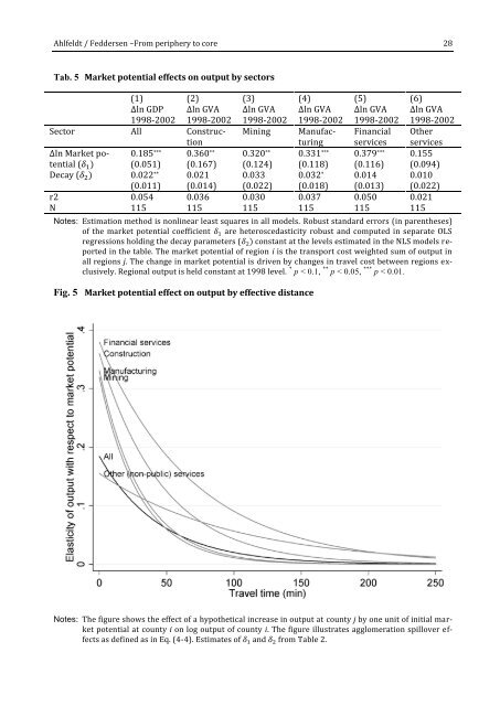
Ahlfeldt / Feddersen –From periphery to core 28Tab. 5 Market potential effects on output by sectors(1) (2) (3) (4) (5) (6)Δln GDP1998-2002Δln GVA1998-2002Δln GVA1998-2002Δln GVA1998-2002Δln GVA1998-2002Δln GVA1998-2002Sector All ConstructionMining ManufacturingFinancialservicesOtherservicesΔln Market potential(δ 1 )0.185 ***(0.051)0.360 **(0.167)0.320 **(0.124)0.331 ***(0.118)0.379 ***(0.116)0.155(0.094)Decay (δ 2 ) 0.022 ** 0.021 0.033 0.032 * 0.014 0.010(0.011) (0.014) (0.022) (0.018) (0.013) (0.022)r2 0.054 0.036 0.030 0.037 0.050 0.021N 115 115 115 115 115 115Notes: Estimation method is nonlinear least squares in all models. Robust standard errors (in parentheses)of the market potential coefficient δ 1 are heteroscedasticity robust and computed in separate OLSregressions holding the decay parameters (δ 2 ) constant at the levels estimated in the NLS models reportedin the table. The market potential of region i is the transport cost weighted sum of output inall regions j. The change in market potential is driven by changes in travel cost between regions exclusively.Regional output is held constant at 1998 level. * p < 0.1, ** p < 0.05, *** p < 0.01.Fig. 5 Market potential effect on output by effective distanceNotes: The figure shows the effect of a hypothetical increase in output at county j by one unit of initial marketpotential at county i on log output of county i. The figure illustrates agglomeration spillover effectsas defined as in Eq. (4-4). Estimates of δ 1 and δ 2 from Table 2.
Page 1 and 2: SERC DISCUSSION PAPER 172From Perip
Page 4 and 5: AbstractWe analyze the economic imp
Page 6 and 7: Ahlfeldt / Feddersen -From peripher
Page 44 and 45: AHLFELDT / FEDDERSEN -FROM PERIPHER

sercdp0172

Create successful ePaper yourself

Delete template?

Save as template?