Defining and Measuring Trophic Role Similarity in Food Webs Using ...

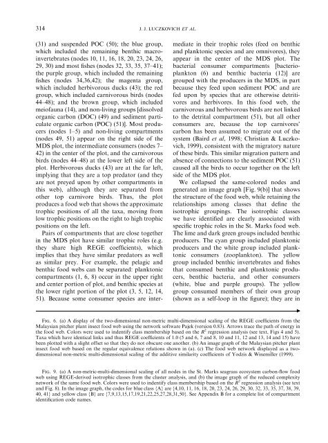
314J. J. LUCZKOVICH ET AL.(31) and suspended POC (50); the blue group,which included the remaining benthic macroinvertebrates(nodes 10, 11, 16, 18, 20, 23, 24, 26,29, 30) and most fishes (nodes 32, 33, 35, 37–41);the purple group, which included the remainingfishes (nodes 34,36,42); the magenta group,which included herbivorous ducks (43); the redgroup, which included carnivorous birds (nodes44–48); and the brown group, which includedmeiofauna (14), and non-living groups [dissolvedorganic carbon (DOC) (49) and sediment particulateorganic carbon (POC) (51)]. Most producers(nodes 1–5) and non-living compartments(nodes 49, 51) appear on the right side of theMDS plot, the intermediate consumers (nodes 7–42) in the center of the plot, and the carnivorousbirds (nodes 44–48) at the lower left side of theplot. Herbivorous ducks (43) are at the far left,implying that they are a top predator (and theyare not preyed upon by other compartments inthis web), although they are separated fromother top carnivore birds. Thus, the plotproduces a food web that shows the approximatetrophic positions of all the taxa, moving fromlow trophic positions on the right to high trophicpositions on the left.Pairs of compartments that are close togetherin the MDS plot have similar trophic roles (e.g.they share high REGE coefficients), whichimplies that they have similar predators as wellas similar prey. For example, the pelagic andbenthic food webs can be separated: planktoniccompartments (1, 6, 8) occur in the upper rightand center portion of plot, and benthic species atthe lower right portion of the plot (3, 5, 12, 14,51). Because some consumer species are intermediatein their trophic roles (feed on benthicand planktonic species and are omnivores), theyappear in the center of the MDS plot. Thebacterial consumer compartments [bacterioplankton(6) and benthic bacteria (12)] aregrouped with the producers in the MDS, in partbecause they feed upon sediment POC and arefed upon by species that are otherwise detritivoresand herbivores. In this food web, thecarnivorous and herbivorous birds are not linkedto the detrital compartment (51), but all otherconsumers are, because the top carnivores’carbon has been assumed to migrate out of thesystem(Baird et al, 1998; Christian & Luczkovich,1999), consistent with the migratory natureof these birds. This similar migration pattern andabsence of connections to the sediment POC (51)caused all the birds to occur together on the leftside of the MDS plot.We collapsed the same-colored nodes andgenerated an image graph [Fig. 9(b)] that showsthe structure of the food web, while retaining therelationships among classes that define theisotrophic groupings. The isotrophic classeswe have identified are clearly associated withspecific trophic roles in the St. Marks food web.The lime and dark green groups included benthicproducers. The cyan group included planktonicproducers and the white group included planktonicconsumers (zooplankton). The yellowgroup included benthic invertebrates and fishesthat consumed benthic and planktonic producers,benthic bacteria, and other consumers(white, blue and purple groups). The yellowgroup consumed members of their own group(shown as a self-loop in the figure); they are inFig. 6. (a) A display of the two-dimensional non-metric multi-dimensional scaling of the REGE coefficients from theMalaysian pitcher plant insect food web using the network software Pajek (version 0.83). Arrows trace the path of energy inthe food web. Colors were used to indentify class membership based on the R 2 regression analysis (see text, Figs 4 and 5).Taxa which have identical links and thus REGE coefficients of 1.0 (5 and 6, 7 and 8, 10 and 11, 12 and 13, 14 and 15) havebeen plotted with a slight offset so that they do not obscure one another. (b) An image graph of the Malaysian pitcher plantinsect food web based on the regular equivalence relations shown in (a). (c) The food web network displayed as a twodimensionalnon-metric multi-dimensional scaling of the additive similarity coefficients of Yodzis & Winemiller (1999).cFig. 9. (a) A non-metric-multi-dimensional scaling of all nodes in the St. Marks seagrass ecosystem carbon-flow foodweb using REGE-derived isotrophic classes from the cluster analysis, and (b) the image graph of the reduced complexitynetwork of the same food web. Colors were used to indentify class membership based on the R 2 regression analysis (see textand Fig. 8). In the image graph, the codes for blue class {A} are {4,10, 11, 16, 18, 20, 23, 24, 26, 29, 30, 32, 33, 35, 37, 38, 39,40, 41} and yellow class {B} are {7,9,13,15,17,19,21,22,25,27,28,31,50}. See Appendix B for a complete list of compartmentidentification code names.