Hubbard Model for Asymmetric Ultracold Fermionic ... - KOMET 337

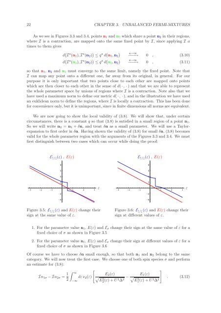
22 CHAPTER 3. UNBALANCED FERMI-MIXTURESAs we see in Figures 3.3 and 3.4, points n 1 and n 3 which share a point n 2 in their regions,where I is a contraction, are mapped onto the same fixed point by I, since applying I atimes to them givesd ( I a (n 1 ), I a (n 2 ) ) ≤ q a d ( ) a→∞n 1 ,n 2 −−−→ 0 , (3.10)d ( I a (n 3 ), I a (n 2 ) ) ≤ q a d ( n 2 ,n 2)a→∞−−−→ 0 , (3.11)so that n 1 , n 2 and n 3 must converge to the same limit, namely the fixed point. Note thatI can map any point onto a different one, far away from its original, in general. For ourpurpose it is only important that two points close to each other are mapped onto pointswhich are then closer to each other in the sense of d( ·, ·) and that we are able to representthe whole parameter space by unions of regions where I is a contraction. Note also that wehave used a maximum norm to define our metric d( ·, ·), and in the illustration we have usedan euklidean norm to define the regions, where I is locally a contraction. This has been donefor convenience only, but it is unimportant, since in finite dimensions all norms are equivalent.We are now going to show the local validity of (3.8). We will show that, under certaincircumstances, there is a constant q so that (3.8) is satisfied in a small region of a point n 1 .So we will write n 2 = n 1 + δn, and treat δn as a small parameter. We will use a Taylorexpansionto first order in δn. Having shown the validity of (3.8) for small δn, (3.8) becomesvalid for the whole parameter region with the arguments of the Figures 3.3 and 3.4. We mustfirst distinguish between two cases which can occur while doing the proof:E ↑/↓ (ε) , E(ε)E ↑/↓ (ε) , E(ε)8866442-3 -2 -1 1 2 3-2ε2-3 -2 -1 1 2 3-2ε-4-4Figure 3.5: E ↑/↓ (ε) and E(ε) change theirsign at the same value of ε.Figure 3.6: E ↑/↓ (ε) and E(ε) change theirsign at different values of ε.1. For the parameter value n 1 , E(ε) and E σ change their sign at the same value of ε for afixed choice of σ as shown in Figure 3.52. For the parameter value n 1 , E(ε) and E σ change their sign at different values of ε for afixed choice of σ as shown in Figure 3.6Of course we have to choose δn small enough, so that both n 1 and n 2 belong to the samecategory. We will now treat the first case. We choose one of both spin species σ and performan estimate for (3.8):In 1σ − In 2σ = 1 ∫ []∞E 2 (ε)dεν d (ε) √2E22 (ε) + U 2 ∆ − E 1 (ε)√ . (3.12)2 E21 (ε) + U 2 ∆ 2−∞