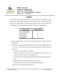
Mathematical modeling

Assume: Z= value of overall measure of performancex j = level of activity j (j=1, 2, ….. , n)c j = increase in Z that result from each unit increase in activity jb i = amount of resource i that is available to activity j (i=1, 2,…, m)a ij = amount of resource i consumed by each unit of activity j.The general form of allocating resources to activities in order to form the generalmathematical model of linear programming is as follows:Resource12.mResources usage per unit of activity1 2 …… nAmount of resource availablea 11 a 12 …… a 1nb 1a 21 a 22 …… a 2nb 2……. .... …… …a m1 a m2 ..….. a mn b mContribution to Z c 1 c 2 ……. c nSo, the general model is to select the values of x 1 , x 2 , ….., x n so as toMaximizeZ = c 1 x 1 + c 2 x 2 + …… + c n x nSubject to a 11 x 1 + a 12 x 2 + …… + a 1n x n ≤ b 1a 21 x 1 + a 22 x 2 + …… + a 2n x n ≤ b 2.a m1 x 1 + a m2 x 2 + …… + a mn x n ≤ b mx 1 ≥ 0, x 2 ≥ 0, …..andx n ≥ 0 non-negativity constraintGenerally, the function being maximized is called the objective function. The first mrestrictions are called the constraints. The x j ≥ 0 restrictions are non-negativity constraints.2.3.3 Solving the Model GraphicallyModels are useful as they allow for a formal definition of a problem and can be useful inthinking about a problem. For a model with only two variables, it is possible to solve theproblem by drawing the feasible region and determining how the objective is optimizedon that region. That process is illustrated here. The purpose of this exercise is to give youintuition and understanding of linear programming models and their solution. In any realapplication, you would use a computer to solve even two variable problems (Excel'sSolver is outlined in the next section to find solutions for linear programming problems).Systems Analysis 17 Dr. Emad Elbeltagi

Note that just graphing the model gives us information we did not have before. It seemsthat the Chip constraint (x 1 + x 2 ≤ 10) plays little role in this model. This constraint isdominated by other constraints. Now, how the optimal solution could be found? Thiscould be done by drawing the objective function line on this diagram. This line representsthe points along which the profit is the same. Since our goal is to maximize the profit, wecan push the objective function line out until moving it any further would result in nofeasible point (Fig. 2.5, z represents the profit). Clearly the optimal profit occurs at pointX. For any value of z, all lines will be parallel as shown in Fig. 2.5. The objectivefunction z = 750x 1 + 1000x 2 can be written in the following form:1000x 2 = -750x 1 + z or x 2 = -750/1000x 1 + z/1000or x 2 = -3/4x 1 + z/1000The last equation called the slop-intercept form of the objective function, demonstratethat the slope of the line is -3/4 (since each unit increase in x 2 changes x 1 by -3/4), wherethe intercept of the line with the x 2 axis is z/1000 (since x 2 = z/1000 when x 1 = 0). Thatfact that the slope is fixed at -3/4 means that all lines constructed in this way are parallel.The variable values at point X represent the intersection point of the two constraints: x 1 +2x 2 ≤ 15 and 4x 1 + 3x 2 ≤ 25.(Optimum solution)Figure 2.5: Finding optimal solutionSystems Analysis 19 Dr. Emad Elbeltagi

By solving the previous two constraints equations, the values of x 1 and x 2 can be easilydetermined: the solution here is x 1 = 1 and x 2 = 7. The optimal decision is to produce1,000 notebooks and 7,000 desktops, for a profit of LE 7,750,000.2.3.4 Terminology of the Model SolutionThe final answer for the problem is always called solution, however in linearprogramming, any values for the decision variables ( x 1 , x 2 , …… ) that satisfies allconstraints are called a solution. So the following definitions are adopted: A feasiblesolution is a solution for which all the constraints are satisfied. An infeasible solution isa solution for which at least one constraint is violated.In the previous example, the points (2, 3) and (1, 6) are feasible solutions, while thepoints (4, 6) and ( -1, 3) are infeasible solutions. The feasible region is the collection ofall feasible solutions. In the example, the feasible region is the entire shaded area asshown in Fig. 2.6. It is possible for the problem to have no feasible solutions. This wouldhave happened in the example if it was required to have a net profit of at least LE 10,000per quarter. This constraint 750x 1 + 1000x 2 ≥ 10000 would eliminate the entire feasibleregion, so no mix of products would be able to produce this profit as shown in Fig. 2.7.(0, 10)(0, 8.3)(0, 7.5)(1, 7)optimumFeasibleregionActiveconstraintInactiveconstraintActiveconstraint(6.25, 0) (10, 0)(15, 0)Figure 2.6: Solution terminologySystems Analysis 20 Dr. Emad Elbeltagi

must contain a bounded feasible region. The bonded region always has CPF [(0, 0); (6.25,0); (1, 7); (0, 7.5)] and solutions with at least one optimal solution; (1, 7) . Thus, if aproblem has exactly one optimal solution, it must be a CPF solution. If the problem hasmultiple optimal solutions, at least two must be CPF solutions.An active constraint is the constraint that share in forming the feasible region, while anin-active constraint is the constraint that doesn’t share in forming the feasible region. Inthe previous example, the following constraints are represents the set of activeconstraints: x 1 + 2 x 2 ≤ 15; 4x 1 + 3x 2 ≤ 25; x 1 ≥ 0 and x 2 ≥ 0, while the x 1 + x 2 ≤ 10 is anin-active constraint (these are shown in Fig. 2.6).2.3.5 Solving Using Solver ProgramRather than the somewhat tedious and error-prone graphical method (which is limited totwo variables), special computer programs can be used to find solutions to linearprogramming models. The most widespread program is Solver, included in all recentversions of the Excel spreadsheet program. Solver, while not a state of the art code is areasonably robust, easy-to-use tool for linear programming. Solver uses standardspreadsheets together with an interface to define variables, objective, and constraints todefine a linear program. Excel Solver add-in optimizes linear and integer problems usingthe simplex and branch and bound methods. It searches for the proper values of modelvariables that minimize or maximize a target cell (objective function), under a set of userspecifiedconstraints. The following is a brief outline and hints for using solver:- Start with entering the data into spreadsheet in some reasonably way.- Create the model in a separate part of the worksheet. Each variable is described inone cell. Solver will eventually put the optimal values in each cell.- The objective is represented by a single cell. The formula that represents theobjective function will be entered in a linear form. The problem modeling of theprevious example in a spreadsheet is shown in Fig. 2.8.- We then have a cell to represent the left hand side of each constraint (again alinear function) and another cell to represent the right hand side (a constant).Systems Analysis 22 Dr. Emad Elbeltagi

Changeable cells(variables)Target cell(objective)Figure 2.8: Problem modeling in Excel- We then select Solver under the Data menu (Excel 2007). This gives a form todefine the linear program. If solver is not available in your Excel program, youmay add it using “Excel Options” then “Add-Ins”.- In the “Set Target Cell" box, select the objective cell and then choose “Max” formaximization or “Min” for minimization option buttons or you may set theobjective to a specific value by choosing “value of” option button (Fig. 2.9).- In the “By Changing Cells", put in the range containing the variable cells.- Next, add the constraints by pressing the “Add" button. The dialog box for addingconstraints appears (Fig. 2.10) and it has three parts for the left hand side, the typeof constraint, and the right hand side. Put the cell references for a constraint in theform, choose the right type, and press “Add". Continue until all constraints areadded including the non-negativity; press “OK" after final constraint (Fig. 2.9).Figure 2.9: Solver interface and settingSystems Analysis 23 Dr. Emad Elbeltagi

Figure 2.10: Adding constraints interface- Push the options button and toggle the “Assume Linear Model" in the resultingdialog box. This tells Excel to call a linear rather than a nonlinear programmingroutine so as to solve the problem more efficiently (Fig. 2.9).- Push the Solve button. In the resulting dialog box, select “Answer" and“Sensitivity". This will put the answer and sensitivity analysis in two new sheets.Ask Excel to “Keep Solver values", and your worksheet will be updated withoptimal values are in variable cells. The complete solution of the problem alongwith the sensitivity analysis report is shown in Fig. 2.11.Figure 2.11: Final solver report of the computer company problemSystems Analysis 24 Dr. Emad Elbeltagi

2.4 Second Example: Market AllocationsA marketing company is planning a one week advertising campaign for their new knife.The ads have been designed and produced and now they wish to determine how muchmoney to spend in each advertising outlet. They have hundreds of possible outlets tochoose from. Let’s consider two outlets: Prime-time TV, and newsmagazines. Theproblem of optimally spending advertising money can be formulated in many ways. Forinstance, given a fixed budget, the goal might be to maximize the number of targetcustomers reached (customer with a reasonable chance of purchasing the product). Analternative approach, which we adopt here, is to define targets for reaching each marketsegment and to minimize the money spent to reach those targets. For this product, thetarget segments are teenage boys, women (ages 40-49), and retired men. Each minute ofprimetime TV and page of newsmagazine advertisement reaches the following number ofpeople (in millions):Outlet Boys Women Men CostTV 5 1 3 600Magazine 2 6 3 500Target 24 18 24Again, the marketing company is willing to know how many units of each outlet topurchase to meet the goals.2.4.1 ModelingThe process of modeling using linear programming is fairly consistent: define thedecision variables, objective, and constraints.Decision Variables: In this case, they are the number of units of each outlet to purchase.Let x 1 be the number of TV spots, and x 2 the number of magazine pages.Objective: Our objective is to minimize the amount we spend: 600x 1 + 500x 2 .Systems Analysis 25 Dr. Emad Elbeltagi

Constraints: We have one constraint for each market segment: we must be certain that wereach sufficient people of each segment. For boys, this corresponds to the constraint: 5x 1+ 2 x 2 ≥ 24. Similar constraints for the other segments give us the full formulation as:Minimize 600x 1 + 500x 2Subject to 5x 1 + 2x 2 ≥ 24x 1 + 6x 2 ≥ 183x 1 + 3x 2 ≥ 24x 1 ≥ 0; x 2 ≥ 02.4.2 Solving the Model GraphicallySince this model has only two variables, we can solve the problem in two ways:graphically and using SOLVER. We start by solving this graphically. The first step is tograph the feasible region, as given in Fig. 2.12. The next step is to plot the objectivefunction line on the diagram: lines representing points that have the same cost. We markthe optimal point with an X (Fig. 2.13). X is the intersection of the two constraints: 5x 1 +2x 2 = 24 and 3x 1 + 3x 2 = 24. Solving these to equations together, the optimal solution isdetermined to be as follows: x 1 = 2.67 and x 2 = 5.33Figure 2.12: Marketing exampleSystems Analysis 26 Dr. Emad Elbeltagi

Figure 2.13: Marketing example showing the optimum solution2.4.3 Solving Using Solver ProgramThe problem formulation on Excel is shown in Fig. 2.14, while the Solver setting isshown in Fig. 2.15. The complete report of the problem solution is shown in Fig. 2.16.Figure 2.14: Problem modeling in ExcelFigure 2.15: Solver settingSystems Analysis 27 Dr. Emad Elbeltagi

Figure 2.16: Final solver report of the marketing problem2.5 Types of Linear Programming SolutionsWhenever a linear programming model is formulated and solved, the result will be one offour characteristic solution types: 1) unique optimal solution, 2) alternate optimalsolutions, 3) no-feasible solution, and 4) unbounded solutions. The following exampleillustrates these different situations.Illustrative exampleA small company produces construction materials for the commercial and residentialconstruction industry. The company produces two products: a universal concrete patchingproduct (CON) and a decorative brick mortar (MORT). The company can sell the CONfor a profit of LE 140/ton and the MORT for a profit of LE 160/ton. Each ton of the CONrequires 2 m 3 of the red clay and each ton produced of the MORT requires 4 m 3 . Amaximum of 28 m 3 of the red clay could be available every week. The machine used toblend these products can work only a maximum of 50 hours per week. This machineblends a ton of either product at a time, and the blending process requires 5 hours tocomplete. Each material must be stored in a separate curing vat, thus limiting the overallproduction volume of each product. The curing vats for CON and MORT have capacitiesof 8 and 6 tons, respectively. What is optimal production strategy for the company giventhis information?Systems Analysis 28 Dr. Emad Elbeltagi

Model formulationFirst we have to decide on decision variables. Let us label the two materials (CON andMORT) 1, and 2, and let x 1 represents the number of tons of CON produced each weekand x 2 represents the number of tons of MORT produced each week. Our objective is tomaximize the profit of these materials, which can be written as:Max total weekly profit, Z = 140x 1 + 160x 2We have constraints for the red clay material, the blending time, and for the curing vatcapacity. This gives the following formulation:Subject to: 2x 1 + 4x 2 ≤ 285x 1 + 5x 2 ≤ 50x 1 ≤ 8x 2 ≤ 6x 1 , x 2 ≥ 02.5.1 Problems Having Unique OptimaThe above illustrative example is solved graphically by plotting the feasible region in thedecision space as shown in Fig. 2.17 and then plotting the objective function on the samegraph. Then, shifting the objective function line in the direction of improvement until itlast intersected the feasible region (Fig. 2.17). In this case, the intersection between thefeasible region and the set points satisfying the equation: 1480 = 140x 1 + 160x 2 , whichconsisted of a single point x 1 = 6 and x 2 = 4. This point is the only point on this line thatsatisfies all constraint equations simultaneously. Consequently, the optimal solution tothe linear program is unique one; the problem is said to have unique optimal solution.2.5.2 Problems Having Alternate OptimaAs shown above, the slope of the objective function is determined by the coefficients thatmultiply the decision variables. For example, if the coefficient of x 2 in the originalobjective functions is decreased to the coefficient of x 1 . The slope of the objectiveSystems Analysis 29 Dr. Emad Elbeltagi

function line becomes steeper. Suppose the objective function becomes as follows: Z =140x 1 + 140x 21480 = 140x 1 + 160x 22x 1 + 4x 2 ≤ 285x 1 + 5x 2 ≤ 50x 1 ≤ 8x 2 ≤ 6(6, 4) Unique optimalsolutionFeasible regionFigure 2.17: Graphical solution of the illustrative example with unique optimal solutionNow, resolve the problem graphically as shown in Fig. 2.18. The intersection of theobjective function line and the feasible region at optimality becomes a line segment (Fig.2.18) and all points on the line connecting the points (6, 4) and (8, 2) give the same valueof the objective function and satisfy the equation 1400 = 140x 1 + 140x 2 . This problemthus has an infinite number of optimal solutions, or is said to have alternate optima.1400 = 140x 1 + 140x 2Feasible region(6, 4)Line segment of alternate optima(8, 2)Figure 2.18: Solution of the illustrative example with multi-optimal solutionsSystems Analysis 30 Dr. Emad Elbeltagi

2.5.3 Problems Having No Feasible SolutionIt is possible that there are no feasible solution for a given problem formulation. This mayoccur when constraints conflict with one another. Or it may occur due to errors inentering problem formulation to a solver. Thus means that there is no specific solutionthat satisfies all constraints together. Assume the following set of constraints:5x 1 + 5x 2 ≤ 50x 1 ≥ 8x 2 ≥ 6Figure 2.19 shows three constraints plotted in decision space in such a way that there isno feasible region formed; the problem is said to be infeasible.Figure 2.19: Graphical solution showing no-feasible region2.5.4 Problems that are UnboundedThe infeasible solution results from problems that are over constrained. In the currentcase, we may encounter a situation where the problem is under constrained. Consider thefollowing set of constraints:5x 1 + 5x 2 ≥ 50x 1 ≤ 8x 1 ≥ 6Systems Analysis 31 Dr. Emad Elbeltagi

In Fig. 2.20, the feasible region is shaded and bounded by three constraints. The objectivefunction line and its direction of improvement are also shown. It is clearly shown that forany feasible solution in this decision space, there is always another one that gives a bettervalue of the objective function such that the objective function for this problem could bemoved upwards and to the right without limit. Such a problem is said to be unbounded.5x 1 + 5x 2 ≥ 50x 1 ≥ 6Unbounded feasible regionx 1 ≤ 8Objective function lineFigure 2.20: Unbounded feasible region2.6 Limitations of Linear Programming ModelingHidden in our models of these problems are a number of assumptions. The usefulness ofa model is directly related to how close reality matches up with these assumptions. Thefirst assumption is due to the linear form of our functions. Since the objective is linear,the contribution to the objective of any decision variable is proportional to the value ofthe decision variable. Producing twice as much of a product produces twice as muchprofit; buying twice as many pages of ads costs twice as much. This is theProportionality Assumption.Furthermore, the contribution of a variable to the objective is independent of the valuesof the other variables. One notebook computer is worth LE750, independent of howmany desktop computers we produce. This is the Additivity Assumption. Similarly, sinceeach constraint is linear, the contribution of each variable to the left hand side of eachconstraint is proportional to the value of the variable and independent of the values of anyother variable.Systems Analysis 32 Dr. Emad Elbeltagi

These assumptions are quite restrictive. We will see, however, that clever modeling canhandle situations that may appear to violate these assumptions. The next assumption isthe Divisibility Assumption: it is possible to take any fraction of any variable. Rethinkingthe Marketing example, what does it mean to purchase 2.67 television ads? It may be thatthe divisibility assumption is violated in this example. Or, it may be that the units aresuch that 2.67 “ads" actually corresponds to 2666.7 minutes of ads, in which case we can“round off" our solution to 2667 minutes with little doubt that we are getting an optimalor nearly optimal solution.The final assumption is the Certainty Assumption: linear programming allows for nouncertainty about the numbers. An ad will reach the given number of people; the numberof assembly hours we give will certainly be available. It is very rare that a problem willmeet all of the assumptions exactly. That does not negate the usefulness of a model. Amodel can still give useful managerial insight even if reality differs slightly from therigorous requirements of the model. For instance, the knowledge that our chip inventoryis more than sufficient holds in our first model even if the proportionality assumptions arenot satisfied completely.2.7 Linear Programming ModelsLinear programming models are found in almost every field of business. The next subsectionsshow a number of problems and how to model them by the appropriate choice ofdecision variables, objective, and constraints.2.7.1 Diet ProblemProblem DefinitionWhat is the perfect diet? An ideal diet would meet or exceed basic nutritionalrequirements, be inexpensive, have variety, and be “pleasing to the palate". How can wefind such a diet? Suppose the available foods are as follows:Systems Analysis 33 Dr. Emad Elbeltagi

FoodServingSizeEnergy(kcal)Protein(g)Calcium(mg)Price(cents/serving)Limit(servings/day)Oatmeal 28 g 110 4 2 3 4Chicken 100 g 205 32 12 24 3Eggs 2 Large 160 13 54 13 2WholeMilk237 cc 160 8 285 9 8CherryPie170 g 420 4 22 20 2Beans 260 g 260 14 80 19 2After consulting with nutritionists, we decree that a satisfactory diet has at least 2000 kcalof energy, 55 g of protein, and 800 mg of calcium. While some of us would be happy tolive on 10 servings of beans, we have decided to impose variety by having a limit on thenumber of servings/day for each of our six foods. What is the least cost satisfactory diet?Problem ModelingFirst we decide on decision variables. Let us label the foods 1, 2, … 6, and let x i representthe number of servings of food i in the diet. Our objective is to minimize cost, which canbe written as: 3x 1 + 24x 2 + 13x 3 + 9x 4 + 20x 5 + 19x 6 . We have constraints for energy,protein, calcium, and for each serving/day limit. This gives the formulation:Minimize: 3x 1 + 24x 2 + 13x 3 + 9x 4 + 20x 5 + 19x 6Subject to: 110x 1 + 205x 2 + 160x 3 + 160x 4 + 420x 5 + 260x 6 ≥ 20004x 1 + 32x 2 + 13x 3 + 8x 4 + 4x 5 + 14x 6 ≥ 552x 1 + 12x 2 + 54x 3 + 285x 4 + 22x 5 + 80x 6 ≥ 800x 1 ≤ 4x 2 ≤ 3x 3 ≤ 2x 4 ≤ 8x 5 ≤ 2x 6 ≤ 2x i ≥ 0 (for all i)Systems Analysis 34 Dr. Emad Elbeltagi

2.7.2 Workforce PlanningProblem DefinitionConsider a restaurant that is open seven days a week. Based on past experience, thenumber of workers needed on a particular day is given as follows:Day Mon Tue Wed Thu Fri Sat SunNumber 14 13 15 16 19 18 11Every worker works five consecutive days, and then takes two days off, repeating thispattern. How can we minimize the number of workers that staff the restaurant?ModelA first attempt at this problem is to let x i be the number of people working on day i. Notethat such a variable definition does not match up with what we need. Some workers willwork both Monday and Tuesday, some only one day, some neither of those days. Instead,let the days be numbered 1 through 7 and let x i be the number of workers who begin theirfive day shift on day i. Our objective is clearly minimize: x 1 + x 2 + x 3 + x 4 + x 5 + x 6 + x 7Consider the constraint for Monday's staffing is 14. Who works on Mondays? Clearlythose who start their shift on Monday (x 1 ). Those who start on Tuesday (x 2 ) do not workon Monday, nor do those who start on Wednesday (x 3 ). Those who start on Thursday (x 4 )do work on Monday, as do those who start on Friday, Saturday, and Sunday. This givesthe constraint: x 1 + x 4 + x 5 + x 6 + x 7 ≥ 14. Similar arguments give a total formulation of:Minimize x 1 + x 2 + x 3 + x 4 + x 5 + x 6 + x 7Subject to x 1 + x 4 + x 5 + x 6 + x 7 ≥ 14x 1 + x 2 + x 5 + x 6 + x 7 ≥ 13x 1 + x 2 + x 3 + x 6 + x 7 ≥ 15x 1 + x 2 + x 3 + x 4 + x 7 ≥ 16x 1 + x 2 + x 3 + x 4 + x 5 ≥ 19x 2 + x 3 + x 4 + x 5 + x 6 ≥ 18x 3 + x 4 + x 5 + x 6 + x 7 ≥ 11x i ≥ 0 (for all i)Systems Analysis 35 Dr. Emad Elbeltagi

2.7.3 Financial PortfolioProblem DefinitionThe optimality of a portfolio depends heavily on the model used for defining risk andother aspects of financial instruments. Here is a particularly simple model that isamenable to linear programming techniques. Consider a mortgage team with LE100,000,000 to finance various investments. There are five categories of loans, each withan associated return and risk (1-10; 1 best):Loan/investment Return (%) RiskFirst Mortgages 9 3Second Mortgages 12 6Personal Loans 15 8Commercial Loans 8 2Government Securities 6 1Any non-invested money goes into a savings account with no risk and 3% return. Thegoal for the mortgage team is to allocate the money to the categories so as to: Maximize the average return per dollar. Have an average risk of no more than 5 (risks taken over the invested moneynot over the saved money). Invest at least 20% in commercial loans. The amount in second mortgages and personal loans combined should be nohigher than the amount in first mortgages.ModelLet the investments be numbered 1…..5, and let x i be the amount invested in investmenti. Let x 6 be the amount in the savings account.The objective is to maximize 9x 1 + 12x 2 + 15x 3 + 8x 4 + 6x 5 + 3x 6Subject to x 1 + x 2 + x 3 + x 4 + x 5 + x 6 = 100,000, 000.Systems Analysis 36 Dr. Emad Elbeltagi

Now, let's look at the average risk. Since we want to take the average over only theinvested amount, a direct translation of this constraint is:3x 1 + 6x 2 + 8x 3 + 2x 4 + x 5 / (x 1 + x 2 + x 3 + x 4 + x 5 ) ≤ 5This constraint is simplified to get the equivalent linear constraint:-2x 1 + x 2 + 3x 3 – 3x 4 – 4x 5 ≤ 0Similarly we need x 4 ≥ 0.2 (x 1 + x 2 + x 3 + x 4 + x 5 )Or -0.2x 1 – 0.2x 2 – 0.2x 3 + 0.8x 4 – 0.2x 5 ≥ 0The final constraint is x 2 + x 3 - x 1 ≤ 0Together with non-negativity, this gives the entire formulation.2.8 Solved Examples2.8.1 Example 1A city public works department is planning for a new water supply project. Waterfrom a nearby aquifer is available in adequate supply, but its hardness level is toohigh unless it is blended with a lower hardness source. The total-kilograms ofhardness per million cubic meters are limited to 1200 in the final blended supply.Water from a distant stream is of sufficient quality, but the cost to pump it is quitehigh. The city is planning to get the water from three sources: the current supply;the aquifer; and the distant stream. The costs to get water (LE) per million cubic (mm 3 ) meters and the hardness in kilogram per m m 3 are given below.Source 1 Source 2 Source 3Cost (LE/m m 3 ) 500 1000 2000Supply limit (m m 3 ) 25 120 100Hardness (Kg/ m m 3 ) 200 2300 700A total of 150 million cubic meter of water is needed per day by the end of tenyears. Formulate a mathematical model to determine the least-cost strategy forsupplying water while ensuring that the water supply remains of acceptable quality.SolutionSystems Analysis 37 Dr. Emad Elbeltagi

Let the variables be as follows:x 1 : millions of cubic meters of water per day to be drawn from source 1x 2 : millions of cubic meters of water per day to be drawn from source 2x 3 : millions of cubic meters of water per day to be drawn from source 3The objective is to minimize the cost of waste supply, c,Min c = 500x 1 + 1000x 2 + 2000x 3The constraints are:x 1 + x 2 + x 3 ≥ 150 (required amount of water)200x 1 + 2300x 2 + 700x 3 ≤ 1200 × 150 (hardness constraint)x 1 ≤ 25 (supply constraint)x 2 ≤ 120 (supply constraint)x 3 ≤ 100 (supply constraint)x 1 , x 2 , x 3 ≥ 02.8.2 Example 2You have been hired to plan a new subdivision development. You are trying toevaluate two options: 200 m 2 or 240 m 2 homes. Each 200 m 2 home will cost LE6,000 and make profit of LE 15,000. Also, each 240 m 2 home will cost LE 9,000and make profit of LE 18,000. The available fund for the new subdivisiondevelopment is LE 450,000. Also, at least one-third of the total number of housesshould be of the 240 m 2 type. Define the decision variables and formulate a linearprogram model to maximize the profit. Solve using the graphical method.SolutionThe variables are the number of 200-m 2 and 240-m 2 homes to be built.x 1 = number of 200-m 2 homes.x 2 = number of 240-m 2 homes.Cost of 200-m 2 home = LE 6,000Cost of 240-m 2 home = LE 9,000Profit produced from each 200-m 2 home = LE 15,000Systems Analysis 38 Dr. Emad Elbeltagi

Profit produced from each 240-m 2 home = LE 18,000Maximum fund available for construction = LE 500,000One-third of the hoses should be from the 240-m 2 type.Maximize 15000x 1 + 18000x 2Subject to 6000x 1 + 9000x 2 ≤ 450000x 2 ≥ 0.33(x 1 + x 2 ) or -0.33x 1 + 0.67x 2 ≥ 0x 1 , x 2 ≥ 0As shown in the following figure, the number of 200-m 2 homes is 43 homes, while thenumber of 240-m 2 home is 21 homes, which satisfies a maximum profit of LE 1,029,399.15000x 1 + 18000x 2 = 10293996000x 1 + 9000x 2 ≤ 450000Feasible regionOptimum solution(43.13, 21.24)-0.33x 1 + 0.67x 2 ≥ 02.8.3 Example 3Resolve example 2.8.2 using the Solver program of Excel.SolutionFirst, set the modelin Excel spreadsheetprogram as follow:The solution is shown in the following figure.Systems Analysis 39 Dr. Emad Elbeltagi

2.8.4 Example 4You have been hired to plan a new subdivision development. A manufacturing firmproduces widgets and distributes them to five wholesalers at a fixed delivered price ofLE 2.50 per unit. Sales forecasts indicate that monthly deliveries will be 2700, 2700,9000, 4500 and 3600 widgets to wholesalers 1-5 respectively. The monthlyproduction capacities are 4500, 9000 and 11,250 at plants 1, 2 and 3, respectively.The direct costs of producing each widget are LE 2 at plant 1, LE 1 at plant 2 and LE1.80 at plant 3. The transport cost of shipping a widget from a plant to a wholesaler isgiven below.Wholesaler 1 2 3 4 5Plant 1 0.05 0.07 0.11 0.15 0.16Plant 2 0.08 0.06 0.10 0.12 0.15Plant 3 0.10 0.09 0.09 0.10 0.16Formulate a linear Programming model for this production and distribution problem.SolutionCost of production of widgets from plant 1Cost of production of widgets from plant 2Cost of production of widgets from plant 3Monthly production capacity from plant 1Monthly production capacity from plant 2Monthly production capacity from plant 3Monthly delivery to wholesaler 1= LE 2/unit= LE 1/unit= LE 1.8/unit= 4500 units= 9000 units= 11250 units= 2700 unitsSystems Analysis 40 Dr. Emad Elbeltagi

Monthly delivery to wholesaler 2Monthly delivery to wholesaler 3Monthly delivery to wholesaler 4Monthly delivery to wholesaler 5= 2700 units= 9000 units= 4500 units= 3600 unitsAssume x ij = number of units shipped from plant i to wholesaler jc ij = cost of shipping a unit from plant i to wholesaler jp i= production cost of a unit at plant iLet the variables be as follows:The variables are to determine the number of units to be shipped from eachproduction plant (the three plants) to each wholesaler (the five wholesalers); x ijThe objective is to determine the number of units produced and shipped from plant ito wholesaler j so that the cost of producing and shipping are minimized, costMin cost = (p 1 +c 11 )x 11 + (p 1 +c 12 )x 12 + (p 1 +c 13 )x 13 + (p 1 +c 14 )x 14 + (p 1 +c 15 )x 15 +(p 2 +c 21 ) x 21 +…………………or min cost = ∑∑( p i + c ij )x ij , i=1, 2, 3 and j=1, 2, 3, 4, 5The constraints are:∑ x i1 ≥ 2700, i=1, 2, 3 (amount to wholesaler 1)∑ x i2 ≥ 2700, i=1, 2, 3 (amount to wholesaler 2)∑ x i3 ≥ 9000, i=1, 2, 3 (amount to wholesaler 3)∑ x i4 ≥ 4500, i=1, 2, 3 (amount to wholesaler 4)∑ x i5 ≥ 3600, i=1, 2, 3 (amount to wholesaler 5)∑ x 1j ≤ 4500, j=1, 2, 3, 4, 5 (Production limit of plant 1)∑ x 2j ≤ 9000, j=1, 2, 3, 4, 5 (Production limit of plant 2)∑ x 3j ≤ 11250, j=1, 2, 3, 4, 5 (Production limit of plant 3)x 1j ≥ 02.8.5 Example 5Systems Analysis 41 Dr. Emad Elbeltagi

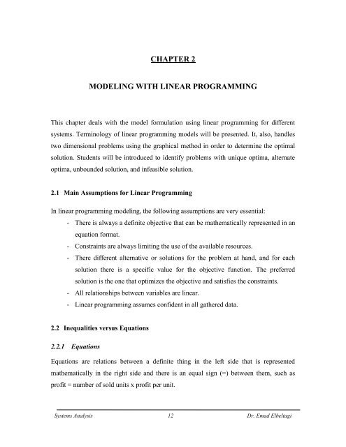
An aggregate mix of sand and gravel must contain no less than 20% no more than30% of gravel. The in situ soil contains 40% gravel and 60% sand. Pure sand may bepurchased and shipped to site at LE 5/m3. A total mix of at least 1000 m3 is required.There is no charge for using in situ material. The objective is to minimize the cost.- Draw the feasible region.- Determine the optimum solution by the graphical method.- Label the active and inactive constraints.SolutionTotal quantity of material needed = 1000 m 3Minimum quantity of gravel in the mix = 0.20 x 1000 = 200 m 3Maximum quantity of gravel in the mix = 0.30 x 1000 = 300 m 3Let the variables be as follows:x 1x 2: Quantity of material from in situ: Quantity of material from outsideThe objective is to minimize the cost, z,Min z = 5x 2The constraints are:x 1 + x 2 ≥ 1000x 214000.4x 1 ≥ 2000.4x 1 ≤ 3001200x 1 , x 2 ≥ 01000Optimum solution:800- x 1 = 750600- x 2 = 250- Amount of gravel = 300 m 3 from in situ- Amount of sand = 700 m 3 ; 450 m 3 from400200(500, 500)(750, 250)in situ and 250 m 3 from outside.02.8.6 Example 6x 10 200 400 600 800 1000 1200Systems Analysis 42 Dr. Emad Elbeltagi

solve the following problem using the graphical method. Compute the value of theobjective function and decision variables at optimality, and indicate which statementbest describes the solution: 1) this linear program has a unique optimnal solution, 2)this linear program has alternate optima, 3) this linear program is infeasible, or 4) thislinear program is unbounded.Minimize Z = 8x 1 + 4x 2Subject to 2x 1 – 2x 2 ≤ 24x 1 - 3x 2 ≥ -64x 1 + 2x 2 ≥ 84x 1 ≥ 44x 2 ≥ 6x 1 , x 2 ≥ 0SolutionThe graphical solution of Example 6 shows that it has alternate optimal solutions whichlie on the line segment between points B (1, 2) and C (1 .25, 1.5) with the objectivefunction equals 16 (optimal solution). It is noted that in this problem, if the objectivefunction is to be maximized, then the problem in this case is said to be unbounded as theobjective function line will move upward with no constraint to limit its movement.Systems Analysis 43 Dr. Emad Elbeltagi

2.9 Exercises1. A plant produces two types of refrigerators, A and B. There are two productionlines, one dedicated to producing refrigerators of Type A, the other to producingrefrigerators of Type B. The capacity of the production line for A is 60 units perday; the capacity of the production line for B is 50 units per day. A requires 20minutes of labor whereas B requires 40 minutes of labor. Presently, there is amaximum of 40 hours of labor per day which can be assigned to either productionline. Profit contributions are LE 20 per Type A produced and LE 30 per Type Bproduced. What should the daily production be? Solve graphically and by Solver.2. A building contractor produces two types of houses: detached and semidetached.The customer is offered several choices of design and layout for each type. Theproportion of each type of design sold in the past is shown in the following table.Design detached semidetachedType AType BType C0.10.40.50.330.67The profit on a detached house and semidetached house is LE 1000 and LE 800respectively. The builder has the capacity to build 400 houses per year. However,an estate of housing is not allowed to contain more than 75% of the total housingas detached. Furthermore, because of the limited supply of bricks available fortype B design, a 200-house limit with this design is imposed. Develop amathematical model for this problem to determine how many detached andsemidetached houses should be constructed in order to maximize profit.3. A concrete manufacturer is concerned about how many units of two types ofconcrete elements to produce during the next time period to maximize profit.Each element of type “A” generates a profit of LE 60, while each element of type“B” produces a profit of LE 40. Two and three units of raw materials are neededto produce one concrete element of type A and B, respectively. Also, four and twounits of time are required to produce one concrete element of type A and BSystems Analysis 44 Dr. Emad Elbeltagi

espectively. If 100 units of raw materials and 120 units of time are available,formulate a linear programming model for this problem to determine how manyunits of each type of concrete elements should be produced to maximize profit.4. A contractor may purchase material from two different sand and gravel pits. Theunit cost of material including delivery from pits 1 and 2 is LE 50 and LE 70 percubic meter, respectively, the contractor requires at least 100 cubic meter of mix.The mix must contain a minimum of 30% sand. Pit 1 contains 25% and pit 2contains 50% sand. If the objective is to minimize the cost of material, define thedecision variables and formulate a mathematical model.- Draw the feasible region- Determine the optimum solution by the graphical method- Label the active and inactive constraints- Use Solver to model and solve this problem5. As the director of waste management, you are trying to plan next year’soperations for the disposal of solid waste. You have three options for disposal:OptionLocal county-owned landfillIncinerationContract landfillDisposal cost (LE/ton)6109There are 300,000 people living in the county with an average of 2.75 kg percapita per day of solid waste. Several constraints are applied to the problem:- The total budget for solid waste disposal is LE 3,000,000.- At least LE 300,000 in disposal income is needed to maintain the local landfill.- At least LE 75,000 in disposal income is needed to maintain the incinerator.- The capacity of the incinerator is 50 ton/day (assume 250 working days).- You don’t want to place in excess of 50% of the waste in the local landfill.Formulate a linear program model to produce an optimal plan for solid wastemanagement.Systems Analysis 45 Dr. Emad Elbeltagi

6. It is required to decide how many tons of pure steel and how many tons of scrapmetal to use in manufacturing an alloy. Pure steel costs LE 300 per ton and scrapLE 600 per ton (larger because the impurities must be skimmed o ff). Thecustomer wants at least 5 tons but will accept a larger order and material loss inmelting and casting is negligible. You have 4 tons of steel and 7 tons of scrap towork with, and the weight ratio of scrap to pure cannot exceed 7/8 in the alloy.You are allocated 18 hours melting and casting time in the mill; pure steelrequires 3 hrs per ton and scrap 2 hrs per ton. Write a linear programming modelfor the problem assuming that the objective is to minimize the total steel and scrapcosts. Then, solve graphically for the amount of pure steel and scrap metal to use.7. Egypt National Bank is open Monday-Friday from 9 am to 5 pm. From pastexperience, the bank knows that it needs the following number of tellers.Time Period 9 - 10 10 - 11 11 - noon noon - 1 1 - 2 2 - 3 3 - 4 4 - 5Tellers Required 4 3 4 6 5 6 8 8The bank hires two types of tellers. Full-time tellers work 9-5 five days a week,except for 1 hour off for lunch, either between noon and 1 pm or between 1 pmand 2 pm. Full-time tellers are paid LE 25/hour (this includes payment for lunchhour). The bank may also hire up to 3 part-time tellers. Each part-time teller mustwork exactly 4 consecutive hours each day. A part-time teller is paid LE 20/hour.Formulate a linear program to meet the teller requirements at minimum cost.8. A manufacturer produces two types of timber frame housing packages (type 1 and2). The operations are highly mechanized and the estimated average time requiredfrom each machine for the manufacturing of each package is given below:PackageMachinesA B CType 1 10 10 40Type 2 30 60 20Systems Analysis 46 Dr. Emad Elbeltagi

In a given period there are 600 hours of machine A time available, 850 hours ofmachine B available, and 800 hours of machine C. The expected profit for theproduction of each unit package is LE 2000 for type 1 and LE 1900 for type 2.Formulate a linear program model that maximizes the profit and determine thenumber of house type produces.9. A Corporation produces three types of sprinkler heads for irrigation applications.The company currently has orders for 600 two-inch heads, 500 three-inch heads,and 800 four-inch heads. Sprinkler heads are made from a copper alloy using amold injection process. The company has four different models of molds availablefor use. The first mold, x 1 , produces 15 two-inch heads per pound of alloy; thesecond, x 2 , produces 20 three-inch heads per pound; the third, x 3 , produces 14three-inch heads and 40 four-inch heads per pound; and the fourth, x 4 , produces10 two-inch heads and 20 four-inch heads per pound. The production managerwants to determine the optimal production method to minimize the amount ofcopper used to meet demand. Formulate the problem as a linear programmingmodel.10. For the following constraint set find:x 1 + x 2 ≤ 3 (1)1 ≤ x 2 ≤ 2 (2)x 1 ≥ 0 (3)a. The feasible region on a graph for the constraint set.b. Label the extreme points.c. If the less than or equal to constraint of Eq. (1) is changed to a strict equality,show the feasible region and label the extreme points.11. Pharma produces two chemicals: A and B. These chemicals are produced via twomanufacturing processes. Process 1 requires 2 hours of labor and 1 lb. of rawmaterial to produce 2 oz. of A and 1 oz. of B. Process 2 requires 3 hours of laborand 2 lb. of raw material to produce 3 oz. of A and 2 oz. of B. Sixty hours of laborand 40 lb. of raw material are available. Chemical A sells for LE 16 per oz. and BSystems Analysis 47 Dr. Emad Elbeltagi

sells for LE 14 per oz. Formulate a linear program that maximizes Pharma'srevenue and solve graphically to find the amount of process 1 and process 2 to beproduced. Hint: Define the amounts of Process 1 and Process 2 used, as yourdecision variables.12. There are two suppliers of pipes with their information as shown below in thetable:Source Unit cost (LE/m) Supply limit(m)12100125100unlimitedAt least 900 meters of pipe is required. The goal is to minimize the total cost ofpipe.a. Find the optimum solution.b. Formulate a mathematical model with the supply of pipe from source No. 2limited to 700 meters.c. Does a solution to part b exist? Use the graph to prove your answer.13. Use the graphical method to solve the following problem;Minimize z = 15x 1 + 45x 2Subject to 2x 1 + 3x 2 ≥ 24 (1)x 1 ≥ 2x 2 (2)x 1 ≥ 5 (3)and x 1 ≥ 0, x 2 ≥ 0It is required to draw the feasible region, and determine the minimum value of zgraphically and the corresponding values of x 1 and x 2 .14. Solve the following problem using the graphical method. Compute the value ofthe objective function and decision variables at optimality, and indicate whichstatement best describes the solution: 1) this linear program has a unique optimnalsolution, 2) this linear program has alternate optima, 3) this linear program isinfeasible, or 4) this linear program is unbounded.Systems Analysis 48 Dr. Emad Elbeltagi

Minimize z = - 4x 1 - 6x 2Subject to - 4x 1 – 5x 2 ≤ - 10- x 1 - 4x 2 ≥ - 12- x 1 ≥ - 4x 2 ≥ 1x 1 , x 2 ≥ 015. Solve the following problem using the graphical method. Compute the value ofthe objective function and decision variables at optimality, and indicate whichstatement best describes the solution: 1) this linear program has a unique optimnalsolution, 2) this linear program has alternate optima, 3) this linear program isinfeasible, or 4) this linear program is unbounded.Minimize z = 10x 1 + 4x 2Subject to 5x 1 – 6x 2 ≤ 305x 1 +2x 2 ≥ 30x 1 ≥ 5x 2 ≥ 2.5x 1 , x 2 ≥ 016. Solve the following problem using the graphical method. Compute the value ofthe objective function and decision variables at optimality, and indicate whichstatement best describes the solution: 1) this linear program has a unique optimnalsolution, 2) this linear program has alternate optima, 3) this linear program isinfeasible, or 4) this linear program is unbounded.Maximize z = 24x 1 + 20x 2Subject to x 1 - x 2 ≥ -43x 1 - 2x 2 ≤ 6x 1 + x 2 ≥ 56x 1 + 5x 2 ≤ 10x 2 ≤ 6x 1 , x 2 ≥ 0Systems Analysis 49 Dr. Emad Elbeltagi

17. A company manufactures two products (A and B) and the profit per unit sold isLE 3 and LE 5 respectively. Each product has to be assembled on a particularmachine, each unit of product “A” taking 12 minutes of assembly time and eachunit of product “B” takes 25 minutes of assembly time. The company estimatesthat the machine used for assembly has an effective working week of only 30hours. Solve the following problem using the graphical method to determine howmuch of each product to produce. Note that, as per the market requirements, everyfive units of product A produced at least two units of product B must be produced.If the company has been offered the chance to hire an extra machine, therebydoubling the effective assembly time available; what is the maximum amount youwould be prepared to pay (per week) for the hire of this machine and why?18. Use the graphical method to solve the following problem;Minimize4a + 5b + cSubject to a + b ≥ 11a - b ≤ 5c - a - b = 07a≥ 35 - 12ba ≥ 0; b ≥ 0; c ≥ 0Systems Analysis 50 Dr. Emad Elbeltagi