Categorification of Donaldson-Thomas invariants via perverse ...

More documents

Recommendations

Info

22 YOUNG-HOON KIEM AND JUN LILemma 4.14. Suppose Ξ α and Ξ β are two rank r orientation bundles over an openU. Then for any x ∈ U, there is an open neighborhood U 0 ⊂ U of x such that thereis a homotopy from Ξ α | U0 to Ξ β | U0 .Proof. We begin with an easy fact. For any finite dimensional subspace W 0 ⊂ W :=T x B/T x X, there is a finite dimensional subspace W ⊂ W, containing W 0 , such thatQ x | W is non-degenerate. Indeed, let N ⊂ W 0 be the null-subspace of Q x | W0 . SinceQ x is non-degenerate, we can find a subspace M ⊂ W such that W 0 ∩ M = 0 andQ x : N × M → C is perfect. Then the space W = W 0 ⊕ M ⊂ W is the desiredsubspace.We now construct the desired homotopy. We first find a finite dimensionalsubspace W ⊂ W so that it contains both Ξ α | x /T x X and Ξ β | x /T x X, and Q x isnon-degenerate on W . Let l = r − d x . We form the Grassmannian Gr(l, W )and its Zariski open subset Gr(l, W ) ◦ as in (4.12) (with Q x in place of q). Thenboth [Ξ α | x /T x X] and [Ξ β | x /T x X] are in Gr(l, W ) ◦ . Because Gr(l, W ) ◦ is a smoothconnected quasi-projective variety, we can find an analytic arc [S t ] ∈ Gr(l, W ) ◦ ,t ∈ [0, 1], such that S 0 = Ξ α | x /T x X and S 1 = Ξ β | x /T x X. We let Ξ t,x be thepreimage of S t under the quotient homomorphismπ x : T x B → T x B/T x X.Then [S t ] form an analytic family of subspaces in T x B, interpolating between Ξ α | xand Ξ β | x .We extend this to an analytic family of orientation bundles in a neighborhood ofx ∈ U. As before, we realize an open neighborhood U 0 ⊂ U of x ∈ U as U 0 = X f0 ,x = 0 ∈ V 0 , for the JS chart (V 0 , f 0 ). Then we have the isomorphism of holomorphicBanach bundles T U0 B ∼ = U 0 × ker(∂ ∗ x) 0,1s . By choosing U 0 sufficiently small, we canfind an ɛ > 0 so that Θ U0 (ɛ) ⊂ Ξ α | U0 , Θ U0 (ɛ) ⊂ Ξ β | U0 , and Θ x (ɛ) = □ −1x (0) 0,1 .Next, for i = α and β, we find l analytic sections s i 1, · · · s i l of T U 0B such thatΘ U0 (ɛ) and s i 1, · · · s i l span Ξ i| U0 . Because s α k (x) and sβ k(x) all lie in π−1 x (W ), wecan find arcs ξ k (t) ∈ πx−1 (W ), analytic in t ∈ [0, 1], such that ξ k (0) = s α k(x) andξ k (1) = s β k (x), and Ξ t,x = Θ x (ɛ) ⊕ C-span ( ξ 1 (t), · · · ξ l (t) ) .Using the isomorphism T U0 B ∼ = U 0 × ker(∂ ∗ x) 0,1s , we can view ξ k (t) as analytic arcsin ker(∂ ∗ x) 0,1s ⊂ Ω 0,1 (adE) s . We then defines t k(y) = ξ k (t) + (1 − t)(s α k (y) − s α k (x)) + t(s β k (y) − sβ k (x)).Clearly, they are analytic in t, and s 0 k (y) = sα k (y) and s1 k (y) = sβ k(y) for all y ∈U 0 . Therefore, by shrinking x ∈ U 0 if necessary, for every t ∈ [0, 1], the sectionss t 1(y), · · · s t l (y) and Θ U 0(ɛ) span a rank r analytic subbundle Ξ pret ⊂ U 0 ×Ω 0,1 (adE) s .Because the arcs ξ k (t) are analytic in t, the family Ξ pret is analytic in t. Finally,because [S t ] all lie in Gr(l, W ) ◦ , by shrinking x ∈ U 0 if necessary,Ξ t := image of Ξ pret under U 0 × Ω 0,1 (adE) s → T U0 Bform an analytic family of orientation bundles providing the desired homotopybetween Ξ α | U0 and Ξ β | U0 . □Proof of Proposition 3.4. We first pick a locally finite cover U α so that each U α hasan orientation bundle Ξ α . For each x ∈ X, we pick an open neighborhood U x ofx ∈ X so that (1) U x ⊂ U α whenever x ∈ U α , and that (2) for every pair α, β with
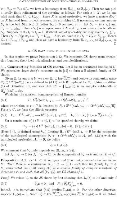
CATEGORIFICATION OF DONALDSON-THOMAS INVARIANTS 23x ∈ U αβ = U α ∩ U β , we have a homotopy from Ξ α | Ux to Ξ β | Ux . Then we can picka locally finite refinement of the covering as follows: For each x ∈ X, we fix anyα(x) such that U x ⊂ U α(x) . Since X is quasi-projective, we have a metric d(·, ·)on X induced from projective space. By shrinking U x if necessary, we may assumeU x is the ball B(x, 2ɛ x ) of radius 2ɛ x > 0 centered at x. Let O x = B(x, ɛ x ) andΞ x = Ξ α(x) | Ox . Then {O x } is an open cover of X and Ξ x is an orientation bundle onO x . Suppose that O x ∩ O y ≠ ∅. Without loss of generality, we may assume ɛ x ≤ ɛ y .Then O x ⊂ B(y, 2ɛ y ) = U y ⊂ U α(y) . Also we have x ∈ O x ⊂ U x ⊂ U α(x) . HenceO x ⊂ U α(x) ∩ U α(y) and thus we have a homotopy from Ξ x | Ox∩O yto Ξ y | Ox∩O yasdesired.□5. CS data from preorientation dataIn this section we prove Proposition 3.12. We construct CS charts from orientationbundles, their local trivializations, and complexifications.5.1. Constructing families of CS charts. Let Ξ be an orientated bundle on U.We generalize Joyce-Song’s construction in [12] to form a Ξ-aligned family of CScharts.Given Ξ, for any x ∈ U, we view Ξ x ⊂ ker(∂ ∗ x) 0,1s and denote its companion spaceΞ ′′x ⊂ Ω 0,1 (adE x ) be as defined in (4.11) with W replaced by Ξ x . Using condition(1) of Definition 3.1, one sees that Ξ ′′ := ∐ x∈U Ξ′′ x is an analytic subbundle ofΩ 0,1X (adE) s−2| U .We define the quotient homomorphism of Banach bundles(5.1) P : Ω 0,1X (adE) s−2| U −→ Ω 0,1X (adE) s−2| U/Ξ ′′ ,whose restriction to x ∈ U is denoted by P x : Ω 0,1 (adE x ) s−2 → Ω 0,1 (adE x ) s−2 /Ξ ′′x.For x ∈ U, we form the elliptic operator(5.2) L x : Ω 0,1 (adE x ) s −→ Ω 0,1 (adE x ) s−2 /Ξ ′′x, L x (a) = P x(□x a + ∂ ∗ x(a ∧ a) ) .For a continuous ε(·) : U → (0, 1) to be specified shortly, we define(5.3) V x = {a ∈ Ω 0,1 (adE x ) s | L x (a) = 0, ‖a‖ s < ε(x)}.(Here ‖ · ‖ s is defined using h x .) Letting Π x : Ω 0,1 (adE x ) s → B be the compositeof the tautological isomorphism ∂ x + · : Ω 0,1 (adE x ) s∼ = Ax (cf. (3.1)) with thetautological projection A x → B, we define(5.4) V x = Π x (V x ).We comment that V x only depends on (Ξ x , h x , ε(x)).Let f x : V x → C (or f x : V x → C) be the composite of V x ↩→ B and cs : B → C.Proposition 5.1. Let U ⊂ X be open and Ξ a rank r orientation bundle onU. Then there is a continuous ε(·) : U → (0, 1) such that the family V x , x ∈U, constructed via (5.3) using ε(·) is a smooth family of complex manifolds ofdimension r, and such that all (V x , f x ) are CS charts of X.Proof. We relate V x to the JS charts by first showing that L x (a) = 0 if and only if(5.5) ∂ ∗ xa = 0 and P x ◦ ∂ ∗ xF 0,2∂ x+a = 0.Indeed, it is immediate that (5.5) implies L x (a) = 0. For the other direction,suppose L x (a) = 0. Since Ξ ′′x ⊂ ker(∂ ∗ x) 0,1s−2 , applying ∂∗ x to L x (a) = 0, we obtain
Page 1 and 2: CATEGORIFICATION OF DONALDSON-THOMA
Page 15: CATEGORIFICATION OF DONALDSON-THOMA
Page 18 and 19: 18 YOUNG-HOON KIEM AND JUN LIwhere
Page 20 and 21: 20 YOUNG-HOON KIEM AND JUN LILemma
Page 24 and 25: 24 YOUNG-HOON KIEM AND JUN LI∂ x
Page 26 and 27: 26 YOUNG-HOON KIEM AND JUN LIWe cal
Page 28 and 29: 28 YOUNG-HOON KIEM AND JUN LIan ope
Page 30 and 31: 30 YOUNG-HOON KIEM AND JUN LIBy can
Page 32 and 33: 32 YOUNG-HOON KIEM AND JUN LIfor so
Page 34 and 35: 34 YOUNG-HOON KIEM AND JUN LI(cf. P
Page 36 and 37: 36 YOUNG-HOON KIEM AND JUN LImixed
Page 38 and 39: 38 YOUNG-HOON KIEM AND JUN LISince
Page 40 and 41: 40 YOUNG-HOON KIEM AND JUN LI8.2. G
Page 42 and 43: 42 YOUNG-HOON KIEM AND JUN LIneed t
Page 44 and 45: 44 YOUNG-HOON KIEM AND JUN LIsuppor
Page 46: 46 YOUNG-HOON KIEM AND JUN LI21. M.

Categorification of Donaldson-Thomas invariants via perverse ...

You also want an ePaper? Increase the reach of your titles

Delete template?

Save as template?