Bayesian analysis of ordinal survey data using the Dirichlet process ...

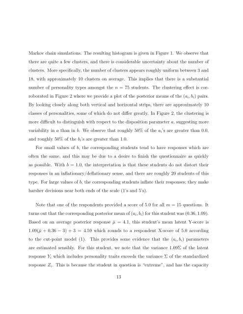
Markov chain simulations. The resulting histogram is given in Figure 1. We observe thatthere are quite a few clusters, and there is considerable uncertainty about the number ofclusters. More specifically, the number of clusters appears roughly uniform between 3 and18, with approximately 10 clusters on average. This implies that there is a substantialnumber of personality types amongst the n = 75 students. The clustering effect is corroboratedin Figure 2 where we provide a plot of the posterior means of the (a i , b i ) pairs.By looking closely along both vertical and horizontal strips, there are approximately 10classes of personalities, some of which do not differ greatly. In Figure 2, the clustering ismore difficult to distinguish with respect to the disposition parameter a, suggesting morevariability in a than in b. We observe that roughly 50% of the a i ’s are greater than 0.0,and roughly 50% of the b i ’s are greater than 1.0.For small values of b, the corresponding students tend to have responses which areoften the same, and this may be due to a desire to finish the questionnaire as quicklyas possible. With b = 1.0, the interpretation is that these students do not distort theirresponses in an inflationary/deflationary sense, and there are roughly 20 students of thistype. For large values of b, the corresponding students inflate their responses; they makeharsher decisions near both ends of the scale (1’s and 5’s).Note that one of the respondents provided a score of 5.0 for all m = 15 questions. Itturns out that the corresponding posterior mean of (a i , b i ) for this student was (0.36, 1.09).Based on an average posterior response ¯µ = 4.1, this student’s mean latent Y-score is1.09(¯µ + 0.36 − 3) + 3 = 4.59 which rounds to a respondent X-score of 5.0 accordingto the cut-point model (1). This provides some evidence that the (a i , b i ) parametersare estimated sensibly. For this student, we note that the variance 1.09Σ of the latentresponse Y i which includes personality traits exceeds the variance Σ of the standardizedresponse Z i . This is because the student in question is “extreme”, and has the capacity13