An expansion method for non-linear Rayleigh waves - FENOMEC

6 P. Panayotaros / Wave Motion 36 (2002) 1–21τ L (u [1] ) ·ˆn =−τ NL (u [0] ,u [0] ) ·ˆn at ∂H, (4.5)and at order α r , r ≥ 2∇·τ L (u [r−1] ) − ρc0 2 ∂2 x 1u [r−1] =τ L (u [r−1] ) ·ˆn =− ∑i+j=r,i,j≥1∑i+j=r,i,j≥1(−∇ · τ NL (u [i−1] ,u [j−1] ) + λ i ρ∂ 2 x 1u [j−1] ) in H, (4.6)τ NL (u [i−1] ,u [j−1] ) ·ˆn at ∂H. (4.7)Thus, u [0] satisfies Eqs. (3.1) and (3.2) for linear traveling waves, while the u [r−1] with r ≥ 2 satisfy the inhomogeneouslinear equation (3.6), with the inhomogeneous part depending on u [0] ,...,u [r−2] and λ 1 ,...,λ r−1 .Inthe inhomogeneous equations, we are looking for pairs u [r−1] , λ r−1 . The way to proceed is standard: first we letu [0] = v [0] be a solution of the homogeneous system (4.3). To solve the order α 2 equations (4.4) and (4.5) for u [1] ,the inhomogeneous part must satisfy the solvability condition (3.7). This is an equation for v [0] and λ 1 . Assumingthat solutions v [0] , λ 1 exist and that the solvability condition is also sufficient, we have a solution u [1] = w [1] +v [1] of(4.4) and (4.5) with w [1] given by the expressions of Appendix A, and v [1] an arbitrary solution of the homogeneouslinear equation (4.3). We can continue this formal procedure to higher order, i.e. determining v [1] and λ 2 from thesolvability condition for the equation for u [2] , decomposing the solution using the particular solution of AppendixA and so on. Assuming that the solvability conditions have solutions, and that they are sufficient for solving theinhomogeneous equation at each order, we may thus write the solution asu = αv [0] + α 2 (v [1] + w [1] ) + α 3 (v [2] + w [2] ) +··· , (4.8)where each v [r−2] , r ≥ 2, is a solution of the homogeneous linear traveling wave equation and is found from thesolvability condition for the order α r equation for u [r−1] , and each w [r−1] , r ≥ 2, is the particular solution of theorder α r inhomogeneous equation for u [r−1] , given in Appendix A.Using (4.3)–(4.7) and the decomposition (4.8) of the displacement u, the solvability condition determining v [r−2]and λ r−1 , r ≥ 2 can be written as∫∫ˆv ∗ (k) · F [r−1] − ˆv ∗ (k) · f [r−1] = 0, ∀k ∈ Z \{0}, (4.9)D∂Dwhere the ˆv i (k) = e ikx 1 ˆv i (k, x 2 ), i.e. as in (3.4), (3.5), andF [r−1] =− ∑(∇ ·τ NL (v [i−1] ,v [j−1] ) +∇·τ NL (v [i−1] ,w [j−1] ) +∇·τ NL (w [i−1] ,v [j−1] )andi+j=r,i,j≥1f [r−1] =− ∑+∇ · τ NL (w [j−1] ,w [j−1] )) + ∑i+j=r,i,j≥1i+j=r,i,j≥1λ i ∂ 2 x 1(v [i−1] + w [j−1] ), (4.10)(τ NL (v [i−1] ,v [j−1] ) ·ˆn + τ NL (v [i−1] ,w [j−1] ) ·ˆn + τ NL (w [i−1] ,v [j−1] ) ·ˆn+τ NL (w [i−1] ,w [j−1] ) ·ˆn). (4.11)Here, we have set w [0] ≡ 0. From (4.10) and (4.11), the solvability condition for the inhomogeneous equation foru [1] is a non-linear equation for v [0] and λ 1 , while the solvability condition for the inhomogeneous equation foru [r−1] , r ≥ 3 is a linear equation for v [r−2] and λ r−1 involving the functions v [0] ,...,v [r−3] ,w [1] ,...,w [r−2] and

8 P. Panayotaros / Wave Motion 36 (2002) 1–21Remark 5.1. For higher order non-linearities, the first solvability condition will also have the form (5.1), onlyinvolving the quadratic non-linearity.An important property of Eq. (5.1) and its Galerkin approximations is homogeneity in c [0] and λ 1 ,ifv [0] = v,λ 1 = λ is a solution of (5.1), then so is ɛv, ɛλ, ∀ɛ ∈ C. Also, for hyperelastic materials, (5.1) describes a constrainedvariational problem:Proposition 5.1.1. The system of Eq. (5.1) is equivalent to∇¯c [0]V(c [0] ) = λ 1 ∇¯c [0]I(c [0] ), (5.3)where the kth component of ∇¯c [0] is [0], k ∈ Z \{0}, and∂¯c k∫V(c [0] ) = W NL (v [0] ,v [0] ,v [0] ), I (c [0] ) = 1 ∫2 ρD2∑Di=12. The Galerkin projections of (5.1) to finite sets J ⊂ Z \{0} are equivalent to[0] V ∇¯c J (c [0]JJ ) = λ 1∇¯c[0]J(∂ x1 v [0]i) 2 . (5.4)I J (c [0]J), (5.5)with V J , I J as in (5.4) with c [0] , v [0] replaced by c [0]J , v[0] J , respectively.Proof.1. From the definition of V and (5.2) we compute for p ∈ Z \{0}∫∂V2∑∂ ¯c p[0] =Vabcdef NL ((∂ x b ˆv a ∗ (p))u c,du e,f + u a,b (∂ xd ˆv c ∗ (p))u e,f + u a,b u c,d (∂ xf ˆv ∗ (p))).Da,b,c,d,e,f =1Passing the derivative to the other side in each of the three terms, we have∂V∂ ¯c p[0]∫=−D∫+∂D2∑ˆv ∗ (p)i=12∑ˆv ∗ (p)i=12∑j=12∑∂ xj2∑φ,χ,ψ,ω=12∑j=1 φ,χ,ψ,ω=1(W NL(W NLij φχψω + W φχijψω NL + W φχψωij NL )u φ,χ u ψ,ωij φχψω + W φχijψω NL + W φχψωij NL )u φ,χ u ψ,ω ˆn j ,which by (2.12) yields∫∫∂V∂ ¯c p[0] =− ˆv ∗ (p) · (∇ ·τ NL (v [0] ,v [0] )) + ˆv ∗ (k) · (τ NL (v [0] ,v [0] ) ·ˆn).D∂DSimilarly,∫∂I2∑∫∂ ¯c p[0] = ρ (∂ xi ˆv i ∗ (p))v[0] i,1 =−ρ ˆv i ∗ (p) · ∂2 x 1v [0] ,Di=1Dso that adding the two terms we have (5.1).

P. Panayotaros / Wave Motion 36 (2002) 1–21 92. The variational formulation for the Galerkin projections follows from the same calculation after replacing v [0]by v [0]J .Corollary 5.2. The Galerkin projections of the first solvability condition (5.1) have non-trivial solutions.Proof. Let c −k =¯c k . We observe that the set I J (c [0]J ) = h>0 is an ellipsoid in R2|J | , |J |=card(J ). SinceV J (c [0]J ) is a smooth real valued function, it will attain its extrema at some points on the ellipsoid and satisfy theGalerkin projection of the solvability condition (5.3) for for appropriate reals λ J 1 .□Remark 5.2. The corollary does not guarantee the existence of Galerkin solutions with λ 1 = 0.By the corollary, one way to approach the problem of finding solutions of (5.1) is to try to understand limits ofsequences of solutions of Galerkin projection of increasing size |J |→∞. In view of the invariance of the Galerkinprojections of (5.1) under rescaling of c [0]J and λJ 1by an arbitrary constant, it appears that we may choose quitearbitrary sequences of Galerkin solutions by changing the scaling factor as we increase the size of the projections.Although this may result useful, in the next section we use the variational interpretation of (5.1) to consider sequencesof solutions belonging to I(c [0]J ) = h, with h fixed as we increase |J |.Although the perturbation theory of the previous section produces an infinite number of solvability conditions,we now see that the second and higher solvability conditions have the same structure. We may use (4.9)–(4.11) towrite the solvability conditions for the inhomogeneous equation obtained at order α r , r>2, as∫− ˆv ∗ (k) · (∇ ·τ NL (v [r−2] ,v [0] ) +∇·τ NL (v [0] ,v [r−2] ))D∫∫+ ˆv ∗ (k) · (τ NL (v [r−2] ,v [0] ) ·ˆn + τ NL (v [0] ,v [r−2] ) ·ˆn) + ρλ 1 ˆv ∗ (k) · ∂x 2 1v [r−2]∂DD∫+ρλ r−1 v ∗ (k) · ∂x 2 1v [0] = G [r−1]k(v [0] ,...,v [r−3] ,w [1] ,...,w [r−2] ,λ 1 ,...,λ r−2 ) (5.6)Dfor all k ∈ Z \{0}. The G [r−1]kare known since it is assumed that we have solved the previous solvabilityconditions and inhomogeneous equations. The left-hand side of (5.6) involves the linearization of the firstsolvability condition (5.1) around a solution v [0] , λ 1 , applied to the unknown v [r−2] , and we may also write(5.6) as∫[(D 1 S [1] (c [0] ,λ 1 ))v [r−2] ] k + ρλ r−1 ˆv ∗ (k) · ∂x 2 1v [0] = G [r−1]k, k ∈ Z \{0} (5.7)Dwith D 1 the derivative with respect to the first variable, [·] k the kth row. Thus to solve the higher order solvabilityconditions we must invert the linearization of the first solvability condition (5.1) around its solution c [0] .The presence of the λ r−1 , r > 3, allows for one null direction. For instance, if we can find a non-trivial solutionv [0] of (5.1) with λ 1 = 0, the homogeneity of (5.1) gives us a line ɛv [0] , ɛ ∈ R, of solutions. However,it may still be possible to adjust the λ r−1 , r > 3, so that the linearization is invertible in the complementarysubspace.Remark 5.3. Note that the addition of higher order non-linear terms in the traveling wave equation will not alterthe general structure of (5.6). Cubic and higher order terms will involve terms v [j] , w [j] with j at most r − 3, andwill thus be absorbed in the right-hand side of G [r−1]k.The variational structure of the higher solvability conditions is expressed by the following statement.

10 P. Panayotaros / Wave Motion 36 (2002) 1–21Proposition 5.2.1. Let c [r−2] be the vector of the coefficients c [r−2]k∈ C, k ∈ Z \{0} of v [r−2] = ∑ k∈Z\{0} c[r−2] kv(k). Then thesolvability condition for the order α r , r>3 inhomogeneous Eq. (4.6), (4.7) is equivalent to∇¯c [r−2]V [r−2] (c [r−2] ) = λ r−1 ∇¯c [r−2]I [r−2] (c [r−2] ), (5.8)where the gradient ∇¯c [r−2] has components [r−2], k ∈ Z \{0}, and∂¯c k∫I [r−2] = ρD2∑i=1(∂ x1 v [r−2]i)(∂ x1 v [0]i). (5.9)For the potential energy V [r−2] , each pair of terms ∇·τ NL (f, g), τ NL (f, g)·ˆn of F [r−1] , f [r−1] in (4.10), (4.11),respectively, is the gradient ∇¯c [r−2] of∫V f,g = (V NL (v [r−2] ,f,g)+ V NL (f, v [r−2] ,g)+ V NL (f,g,v [r−2] )), (5.10)Dalso, each term λ i ∂x 2 1f in (4.10) is the gradient ∇¯c [r−2]v [0] ,...,v [r−3] ,w [1] ,...,w [r−2] , where∫I ˜ [r−2]f=−ρD2∑i=1of 1 2 λ i ˜ I [r−2]fif f = v [r−2] , and λ i ˜ I [r−2]fif f =(∂ x1 v [r−2]i)(∂ x1 f). (5.11)2. The variational structure of the Galerkin projections is given by (1), with V [r−2] , I [r−2] replaced by V [r−2] (c [r−2]J ),I [r−2] (c [r−2]J ), respectively.Proof. The proposition follows by a calculation similar to the one used in showing Proposition 5.1, i.e. we integrateby parts to transfer derivatives on ˆv ∗ (k) to the other terms of the area integrals.□In contrast to the first solvability condition, here the variational structure does not automatically guarantee theexistence of solutions for the Galerkin projections. The constraint I [r−2] = h ∈ R is a hyperplane, while thefunction V [r−2] is quadratic in v [r−2] (see e.g. (5.10) with f = v [0] , g = v [r−2] ), and there is no a priori reason toexpect that V [r−2] has a convex quadratic part. In the case where the first solvability condition has solutions withλ 1 = 0, the constraint I [r−2] = h eliminates a null direction.6. Numerical study of the first solvability conditionIn this section, we study the first solvability condition numerically for three different hyperelastic materials,namely the St. Venant-Kirchhoff material, and two simpler but less physical models.According to the theory of elasticity, the assumptions of material frame indifference and isotropy (see e.g. [15],Chapter 4) which imply that the potential energy density W of a two-dimensional hyperelastic material is a functionof the trace of the matrices E, E 2 and E 3 ,orW = W(tr E, tr E 2 , tr E 3 ), where E = 1 2 (∇u + (∇u)T + (∇u) T ∇u) (6.1)is the strain tensor. We may also assume that the potential energy density does not involve terms that are linear inthe displacement u. This way the trivial displacement u ≡ 0 is a solution of the equations of motion.

P. Panayotaros / Wave Motion 36 (2002) 1–21 11The first non-linearity we choose corresponds to one of the simplest models satisfying the above constraints, andis specified byW = 1 2 λ(tr E)2 + µ tr E 2 (6.2)(this is the St. Venant-Kirchhoff material, see [15], Chapter 4). The quadratic terms in (6.2) give us the quadraticpotential energy density W L of (2.9), while the first solvability condition involves the cubic terms in (6.2). Thesimpler models we will consider correspond to the potential energy densities W = W L + W NL with W L as in (2.9)andW NL =4 1 (λ + µ)u 1,1u 2 1,2 , and W NL =4 1 (λ + µ)(u 1,1u 2 1,2 + u 2,2u 2 2,1 ), (6.3)respectively. Note that these models are not consistent with isotropy.To simplify the first solvability conditions, we will look for traveling wave solutions of (2.4) and (2.5) satisfyingu 1 (−x 1 ,x 2 ) =−u 1 (x 1 ,x 2 ), and u 2 (−x 1 ,x 2 ) = u 2 (x 1 ,x 2 ), ∀(x 1 ,x 2 ) ∈ ˜D. (6.4)These parities are specific to the fundamental domain ˜D of Section 2. We easily check that the traveling waveequation (2.4) for the non-linearities we are considering, as well as the linear equations of the perturbativescheme of Section 4 are compatible with the parities of (6.4). The periodicity and decay conditions are (2.5)and (2.6), respectively. Solutions of the linear traveling wave equation with the parities (6.4) will have theformv [0]1 (x 1,x 2 ) =where∞∑∞∑a p sin px 1 A(p, ˆ x 2 ), v [0]2 (x 1,x 2 ) = a p cos px 1 ˆB(p, x 2 ),p=1p=1ˆ A(p, x 2 ) =−i ˆv 1 (p, x 2 ), ˆB(p, x 2 ) =−ˆv 2 (p, x 2 ), (6.5)i.e. see (3.4) and (3.5), and the coefficients a p ∈ R, ∀p ∈ Z + . The solvability condition for the inhomogeneouslinear equations is (3.7), with ˆv ∗ (k, x 2 ) replaced by [ A(k, ˆ x 2 ), − ˆB(k, x 2 )] and the ˆF i (k, x 2 ), fˆi (k, x 2 ) replaced bythe sine (i = 1) and cosine (i = 2) transforms of F i , f i , respectively. Furthermore, the first solvability conditionhas the variational formulation∂ ap V(a)= λ 1 ∂ ap I(a), p ∈ Z + , (6.6)where the components a p , p ∈ Z + of the vector a are as in (6.6). The functions V(a)and I(a)are given by (5.4),with the linear solutions v [0] as in (6.5).With the above information we can write the solvability condition in spectral form in a straightforward mannerby evaluating V(a), I(a)and the variational equation (6.6). The potential energy V(a)for a general cubic potentialenergy density W NL of the form given in (2.10) will beV(a)=∞∑p 2 >p 3 ≥1+∞∑p 2 ,p 3 ≥1π(p 2 − p 3 )p 2 p 3 a p2 −p 3a p2 a p32 C −(p 2 − p 3 ,p 2 ,p 3 )π(p 2 + p 3 )p 2 p 3 a p2 +p 3a p2 a p32 C +(p 2 + p 3 ,p 2 ,p 3 ). (6.7)For instance, for the first model non-linearity of (6.3) we have C + (q,r,s)= C − (q,r,s)withC − (q,r,s)= λ + µ I 114′ 1 ′(q,r,s)≡ λ + µ ∫ ∞A(q, ˆ x 2 ) A ˆ ′ (r, x 2 ) A ˆ ′ (s, x 2 ) dx 2 , (6.8)4rs0q,r,s ∈ Z + (derivatives are with respect to x 2 ). The coefficients I 11 ′ 1 ′(q,r,s)are given in Appendix B.

12 P. Panayotaros / Wave Motion 36 (2002) 1–21For the kinetic energy part I(a)we haveI(a) = M ∞∑pa 2 p (6.9)2p=1(the constant M is in Appendix B), so that by (6.7) the solvability condition (6.6) takes the formG p (a, λ 1 ) =p−1∑p 1 =1pp 1 (p − p 1 )a p1 a p−p1 K p,p1 +∞∑pp 1 (p + p 1 )a p1 a p+p1 Λ p,p1 − λ 1 Mpa p = 0,p 1 =1p ∈ Z + (6.10)For the first non-linearity of (6.2), we haveK p,p1 =(λ + µ)π(I 118′ 1 ′(p − p 1,p,p 1 ) − I 11 ′ 1 ′(p, p − p 1,p 1 )), (6.11)(λ + µ)πΛ p,p1 = (I 118′ 1 ′(p, p + p 1,p 1 ) + I 11 ′ 1 ′(p 1,p+ p 1 ,p)−I 11 ′ 1 ′(p + p 1,p,p 1 ) − I 11 ′ 1 ′(p + p 1,p 1 , p)). (6.12)The coefficients C ± (q,r,s)for the other non-linearities are in Appendix B. They similarly involve triple integralsof the functions A(q, ˆ x 2 ), ˆB(q, x 2 ) of (6.5) and their derivatives, and are sums of terms α/(βq + γr + δs),with α, β, γ, δ ∈ R constants depending on A and B. The denominators in the coefficients K p,p1 , Λ p,p1 arebounded away from zero uniformly in the allowed integers p, p 1 , so that the coefficients are well-defined. Theseobservations also apply to the coefficients C ± (q,r,s), K p,p1 , and Λ p,p1 obtained for general non-linearities thathave the form of (2.10). We can see this by counting the number of derivatives in the cubic potential energyterms.To study the first solvability condition (6.10) numerically, we consider the Galerkin approximations of (6.7) and(6.10) for the vectors a N = [a1 N ,aN 2 ,...,aN N ] ∈ RN , with the necessary modifications in the summations. It is alsoconvenient to introduce the vectors ã N with components ãpN = paN p , p = 1,...,N. Expressing the LagrangianL(a N ) = V(a N ) − λ N 1 I(aN ) and the Galerkin projection G N p (aN ,λ N 1) = 0,p = 1,...,N of (6.10) in the tildevariables we haveG N p (aN ,λ N 1 ) = ∂ a pL N (a N ,λ N 1 ) = p∂ ã pL N (ã N ,λ N 1 ) ≡ p ˜G N p (ãN ,λ N 1 ) = 0, (6.13)p = 1,...,N, and it is sufficient to solve numerically the equation ˜G N p (ãN ,λ N 1) = 0, p = 1,...,N. By Corollary5.2, the Galerkin projections of the first solvability condition have non-trivial solutions and to find them we setλ N 1= 1 and solve numerically˜G N p (ãN , 1) = 0, p = 1,...,N. (6.14)Letting ˜β N = [ ˜β1 N ,..., ˜βN N ] ∈ RN be a non-trivial solution of (6.14), the vector γ N with components⎛⎞−1/2γpN = ⎝ M N∑ 12 p ( ˜β p N )2 ⎠ p −1 ˜β p N , p = 1,...,N (6.15)p=1satisfies the Galerkin projection of (6.10) with N modes, i.e. we have⎛⎞−1/2G N p (γ N ,λ N 1 ) = 0, p = 1,...,N, with λN 1 = ⎝ M N∑ 12 p ( ˜β p N )2 ⎠ . (6.16)p=1

P. Panayotaros / Wave Motion 36 (2002) 1–21 13Moreover,I N (γ N ) = M 2N∑p(γp N )2 = 1. (6.17)p=1Remark 6.1. The choice of the constraint I N (a N ) = 1 used here is arbitrary, we can also work with I N (a N ) = hfor any h>0. We can rescale γ N and λ N 1by h to also obtain a solution of the N-mode Galerkin projection of thefirst solvability condition. Even though the first solvability condition has no intrinsic scale, it is natural to impose ascale on the lowest order displacement u [0] . This way the assumption on the smallness of the parameter α becomesmeaningful (the scale of γ N and λ N 1can be absorbed in α).For the purpose of the numerical study, the choice of scale is useful for comparing solutions of the differentGalerkin projections. To find candidates for solutions of (6.10), we consider Galerkin projections with N 1

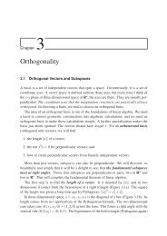
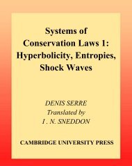
14 P. Panayotaros / Wave Motion 36 (2002) 1–21and find numerically a solution γ N 1, λ N 11 . Then to increase the number of modes from N i to N i+1 , we applyNewton’s iteration for the equation ˜G N i+1p (ã N i+1, 1) = 0, p = 1,...,N i+1 using as initial condition the vector[γ N 1i,...,γ N iN i, 0,...,0] ∈ R N i+1, and obtain (after rescaling the numerical result) γ N i+1 and λ N i+11. Although wecannot control the dynamics of Newton’s iteration, it is reasonable to expect that γ N i, λ N i1 and γ N i+1, λ N i+11will begetting closer as we increase N i .Remark 6.2. The sequence of Fourier coefficient vectors β N i= [γ N i1 ,...,γN iN i, 0,...] obtained from the Galerkinsolutions are bounded in l 2 since ∑ ∞p=1 p(β N ip ) 2 = 1, ∀N i . Therefore, there will be subsequences of {β N i} ∞ i=1that converge weakly in l 2 . Also the corresponding boundary values v [0]1 , v[0] 2of the displacement given by (6.5)will converge weakly in L 2 (S 1 ), and H 1/2 (S 1 ). However, these notions of convergence do not necessarily implythat the limits are non-trivial.Remark 6.3. We will not seek solutions with λ 1 = 0 in this work. The non-invertibility of the linearization of thefunction G(a, 0) in (6.10) around such solutions will likely require that λ i ≠ 0 for i>1, and we plan to considerthis case in the future.Fig. 2. (a) and (b) shows the surface displacement and horizontal component v [0]1 (x 1, 0) of 120, 500 modes, respectively, for second non-linearityof (6.3); (c) and (d) shows the surface displacement and vertical component v [0]2 (x 1, 0) of 120, 500 modes, respectively, for second non-linearityof (6.3) (multiply by 1.47).

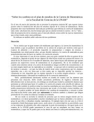
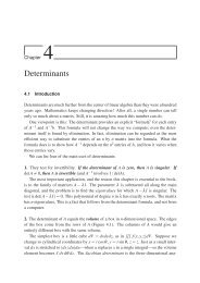
P. Panayotaros / Wave Motion 36 (2002) 1–21 15The numerical results that follow were obtained following the above procedure, and solving (6.14) using the NAGlibrary implementation of the hybrid Newton–Raphson method of [16]. The computed Fourier coefficients of thesurface displacement are normalized as in (6.15). By (6.10), to obtain numerical values for the surface displacement(e.g. ν = 0.28 for glass, ν = 0.28and λ 1 we need to specify the Poisson’s ratio ν =2 1 (λ/(λ+µ)), and we set ν = 4 1for iron, see [15], p. 129). The Rayleigh speed for ν =4 1 is approximately c2 0 = 0.845(µ/ρ).We found two types of sequences of numerical solutions. First, we see sequences where the computed surfacedisplacements v [0]1 (x 1, 0), v [0]2 (x 1, 0) approach definite nontrivial shapes as we increase the number of modes. Thecorresponding sequences λ N i1also seem to approach a limit. The conjectured limits are candidates for solutions ofthe first solvability condition. The shapes of some of the surface displacements obtained numerically for the firstand second non-linearities of (6.3), and for the the St. Venant-Kirchhoff material of (6.2) are shown in Figs. 1–3.Also, the values of λ 1 corresponding to the solutions of Figs. 1–3 are shown in Fig. 6(a)–(c). Evidently, there aresequences of surface displacements and λ 1 with possible non-trivial limits for all three non-linearities considered.An interesting feature of the numerical solutions is the appearance of well-defined cusps in v [0]1 (x 1, 0) for all thenon-linearities considered. On the other hand, v [0]2 (x 1, 0) appears to be differentiable. The numerical solutions alsoFig. 3. (a) and (b) shows surface displacement and horizontal component v [0]1 (x 1, 0) of 300, 500 modes, respectively, St. Venant-Kirchhoffmaterial of (6.2); (c) and (d) shows surface displacement and vertical component v [0]1 (x 1, 0) of 300, 500 modes, respectively, St. Venant-Kirchoffmaterial of (6.2) (multiply by 1.47).

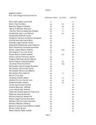
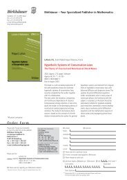
16 P. Panayotaros / Wave Motion 36 (2002) 1–21Fig. 4. (a) and (b) shows coefficients pγ N ip , N i = 200, 500 respectively, solution of Fig. 3.exhibit small oscillations that decrease in scale and amplitude as we increase the size of the Galerkin truncation.This oscillatory behavior can be better appreciated by looking at Fig. 4(a) and (b) where we plot p vs. pγ N ip for threeN i -mode truncations. The γ N ip in Fig. 4(a) and (b) are the Fourier coefficients for the non-linearity of Fig. 3(a)–(d).The tails in pγ N ip are apparently moving to the right with almost constant amplitude as we increase the numberof modes N i , so that γ N iN i∼ p −1 . These features are common to the Fourier coefficients of all the numericalsolutions of this first type, and are evidence that the weak L 2 limits of the surface displacements are non-trivial.It is also possible that we have stronger convergence, e.g. in L 2 (S 1 ), and it is also interesting to see whetherthere is a way to filter out the small-scale oscillations. A more qualitative comparison of the surface displacementsshown is also possible. For instance, evaluating the surface displacements at 2500 uniformly distributed pointsin [−π, π] we see that the difference between the horizontal and vertical displacements obtained using 400 and500 modes is bounded by 2 × 10 −2 for the solutions of Fig. 1(a)–(d), and by 2 × 10 −3 for the solutions ofFigs. 2 and 3(a)–(d). The pointwise difference is in all cases oscillatory and its integral over [−π, π] isintherange 10 −6 –10 −5 .Remark 6.4. The surface displacements we found are reminiscent of those reported in [PT] for a differentnon-linearity. The number of modes used in that work was smaller (∼ 25), and the (possible) cusps were notresolved. It also appears that, at least for the models considered here, the main qualitative features of the numericalsolutions do not depend on the details of the non-linearity.

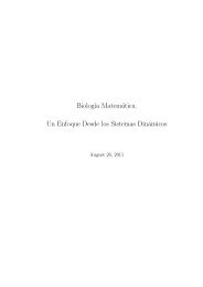
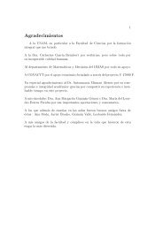
P. Panayotaros / Wave Motion 36 (2002) 1–21 17Remark 6.5. Despite the presence of the cusps at the boundary, (6.15) implies that the lowest order elasticdisplacement v [0] (x 1 ,x 2 ) we obtain from the computed surface displacement is smooth inside the domain.We have also found a second type of sequences of Galerkin solutions that seem to converge weakly in L 2 (S 1 )to the trivial solution. A typical example is shown in Fig. 5(a)–(d). The particular example was found for the St.Venant-Kirchhoff material, but similar numerical solutions were also found for the other non-linearities. In thesesequences, the surface displacement has small-scale oscillations that become finer decreasing slowly in amplitude,as well as spikes that become more and more concentrated as we increase the number of modes. Also, for thistype of numerical solutions the λ N i1do not seem to approach any limit. The λ N i1corresponding to the sequence ofsolutions of Fig. 5 is shown in Fig. 6(d).The accuracy of the numerical solutions presented is indicated by the vector of residuals ˜G N p (xN c , 1), p =1,...,N of the numerical solutions xcN of (6.15). Since, however, lim x→0 ˜G N (x, 1) = 0, it is more meaningful toconsider the vector of relative residuals [ ˜G N p ( ˜xN c , 1)]−1 ˜G N p (xN c , 1), p = 1,...,N, where ˜xN c has the same size asxc N , e.g. in practice we get ˜xN c by changing the sign of a few components of xc N . For the solutions correspondingto all the figures shown, all the components of the relative residuals were bounded by 10 −7 –10 −6 . These numbersFig. 5. (a) and (b) shows surface displacement and horizontal component v [0]1 (x 1, 0) of 160, 500 modes, respectively, St. Venant-Kirchhoff materialof (6.2); (c) and (d) shows surface displacement and vertical component v [0]1 (x 1, 0) of 160, 500 modes, respectively, St. Venant-Kirchhoff materialof (6.2) (multiply by 1.47).

18 P. Panayotaros / Wave Motion 36 (2002) 1–21Fig. 6. Values of λ N i1 for Galerkin approximations with N i modes: (a) solution of Fig. 1; (b) solution of Fig. 2; (c) solution of Fig. 3; (d) solutionof Fig. 5.also agree with the condition for terminating the iteration successfully, i.e. with the relative residuals smaller thanthe square root of the machine accuracy.7. DiscussionWe have considered the problem of traveling surface elastic waves in the half-plane and extended the perturbativeapproach of Parker and Talbot, and Hunter [2,3] to higher order. Our extended scheme is formally equivalentto a perturbative implementation of the Liapunov–Schmidt method, and is also related to Signorini’s method instatic elasticity. The analog of the bifurcation equation is an infinite set of solvability conditions that involve thevalues of the displacement at the surface, and we also observed that for hyperelastic materials the solvabilityconditions are constrained variational problems. In this work, we focused on the first solvability condition. Wenoted that the Galerkin approximations of the first solvability condition must posses solutions, and our numericalresults suggest that there exist sequences of Galerkin solutions with non-trivial limits; such limits are candidates fornon-trivial solutions of the first solvability condition. The Galerkin solutions obtained numerically rather quicklytend to surface displacements of a well-defined shape, although the conjectured convergence is rather slow. Thus,although we consider that our work gives stronger numerical evidence for the existence of non-trivial solutions

P. Panayotaros / Wave Motion 36 (2002) 1–21 19to the first solvability condition than earlier studies, we believe that further improvements are possible and thatthe existence question should also be understood theoretically. It would also be useful (and possibly related tothe existence question) to see whether we can devise a numerical scheme filtering out the small-scale oscillationswe saw.The second step in pursuing the expansion method we described will be to numerically examine the invertibilityof the first solvability condition around its solutions, and the possibility of constructing higher order corrections tothe approximate solutions presented here. A positive result would give further evidence for the existence of travelingwave solutions, although proving existence using the present constructive approach seems difficult at this point, andother strategies may be more practical.Further, dynamical questions can be addressed by considering the asymptotic evolution equation derived byHunter and Parker [3,9]. For instance, one may ask whether the conjectured traveling wave solutions are stable.Instabilities of several types are possible, e.g. to shocks or to radiation (in an extended framework where othermodes are included). Another question is whether arbitrary smooth initial data lead to the formation of cusps andthen shocks. In the neighborhood of a cusp one expects very large forces, so that such loss of regularity phenomenamay have an interesting physical interpretation, relating non-linear effects to the appearance of small-scale cracksnear the surface of solids.AcknowledgementsI would like to thank R. de la Llave, T. Minzoni, A. Olvera and P. Padilla for their helpful discussions andcomments.Appendix AAssuming that the solvability conditions (3.8) and (3.9) are satisfied, the general solution of the inhomogeneouslinear system for the Fourier coefficients û i (k, x 2 ), k ∈ Z, of the displacement isû i (k, x 2 ) = ŵ i (k, x 2 ) + c k ˆv i (k, x 2 ), i = 1, 2, (A.1)where ˆv i (k, x 2 ), i = 1, 2 are the solutions of the homogeneous system given by (3.4) and (3.5), c k ∈ C, andŵ i (k, x 2 ) is a solution of the inhomogeneous system given for k ∈ Z + \{0} by∫ x2ŵ 1 (k, x 2 ) =−iA e −kAx e kAs)2(− iµ−10 2k A 2 − 1 ˆF (λ + 2µ)−11 (k, s) +A(B 2 − 1) ˆF 2 (k, s) ds∫ ∞−iA e kAx e −kAs)2(− iµ−1x 22k A 2 − 1 ˆF (λ + 2µ)−11 (k, s) −A(B 2 − 1) ˆF 2 (k, s) ds[ ∫ x2+i e −kBx e kBs (2iµ−1)2k B(A 2 − 1) ˆF (λ + 2µ)−11 (k, s) − ˆFB 2 2 (k, s) ds− 1− A2 + 12B−0∫ ∞e −kBx 20 2k−i e kBx 2∫ ∞e −kAx 20 2k( iµ−1A 2 − 1 ˆF 1 (k, s) +)(λ + 2µ)−1A(B 2 − 1) ˆF 2 (k, s) ds)(− iµ−1A 2 − 1 ˆF (λ + 2µ)−11 (k, s) +A(B 2 − 1) ˆF 2 (k, s)∫ ∞e −|k|Bsx 22k( iµ−1A 2 − 1 ˆF 1 (k, s) +(λ + 2µ)−1B 2 − 1ds − iµ−1 f ˆ ]1 (k)2kB)ˆF 2 (k, s) ds,(A.2)

20 P. Panayotaros / Wave Motion 36 (2002) 1–21∫ x2ŵ 2 (k, x 2 ) = e −kAx e kAs)2(− iµ−10 2k A 2 − 1 ˆF (λ + 2µ)−11 (k, s) +A(B 2 − 1) ˆF 2 (k, s) ds∫ ∞−e kAx e −kAs)2(− iµ−1x 22k A 2 − 1 ˆF (λ + 2µ)−11 (k, s) −A(B 2 − 1) ˆF 2 (k, s) ds[ ∫ x2−B e −kBx e kBs)2(− iµ−10 2k B(A 2 − 1) ˆF (λ + 2µ)−11 (k, s) + ˆFB 2 2 (k, s) ds− 1∫− A2 + 1 ∞e −kAx )2(− iµ−12B 2k A 2 − 1 ˆF (λ + 2µ)−11 (k, s) −A(B 2 − 1) ˆF 2 (k, s) ds−0( iµ−1∫ ∞e −kBx 20 2k∫ ∞e −kBs−B e kBx 2x 2A 2 − 1 ˆF 1 (k, s) +2k( iµ−1A 2 − 1 ˆF 1 (k, s) +)(λ + 2µ)−1A(B 2 − 1) ˆF 2 (k, s)(λ + 2µ)−1B 2 − 1]ds − iµ−1 fˆ1 (k)2kB)ˆF 2 (k, s) ds,(A.3)and for k = 0by∫ ∞[∫ ∞ŵ 1 (0,x 2 ) =−iµ −1x 2 t]ˆF 1 (0,s)ds dt,∫ ∞[∫ ∞ŵ 2 (0,x 2 ) = (λ + 2µ) −1x 2 t]ˆF 2 (0,s)ds dt.(A.4)For k ∈ Z − , ŵ i (k, x 2 ) = w ∗ i (k, x 2).Ifthe ˆF i (k, x 2 ), i = 1, 2,k ∈ Z are continuous and decay at least polynomially,the above expressions give well-defined solutions of the inhomogeneous system.Appendix BThe coefficients I 11 ′ 1 ′(q,r,s)defined in (6.8) are given by(I 11 ′ 1 ′(q,r,s)= −A 4 1q + r + s + 2A4 B 1(A 2 + 1) (q + r)A + sB + 2A4 B 1(A 2 + 1) (q + s)A + rB− 4A3 B 2 1(A 2 + 1) 2 qA + (r + s)B + 2A5 1(A 2 + 1) (r + s)A + qB − 4A4 B 1(A 2 + 1) 2 rA + (q + s)B)−4A4 B 1(A 2 + 1) 2 sA + (q + r)B + 8A3 B 1(A 2 + 1) 3 . (B.1)q + r + sThe coefficients C ± (q,r,s) in the potential energy V of (6.7) for the other non-linearities are as follows: for thesecond non-linearity of (6.3) we haveC − (q,r,s)= C + (q,r,s)=4 1 (λ + µ)(I 11 ′ 1 ′(q,r,s)+ I 222 ′(q, r, s)),(B.2)while for the St. Venant-Kirchhoff non-linearity of (6.2) we haveC ∓ (q,r,s)=2 1 (λ + 2µ)(I 11 ′ 1 ′(q,r,s)+ I 222 ′(q,r,s)+ I 111(q,r,s)+ I 2 ′ 2 ′ 2 ′(q,r,s)±I 122 (q,r,s)∓ I 2 ′ 1 ′ 1 ′(q,r,s))+2 1 λ(I 112 ′(q,r,s)+ I 12 ′ 2 ′(q,r,s))+ 2 1 µ(∓I 11 ′ 2(q,r,s)− I 21 ′ 2 ′(q, r, s)). (B.3)

P. Panayotaros / Wave Motion 36 (2002) 1–21 21Letting the subscripts φ, χ, ψ range over the symbols 1, 1 ′ ,1 ′′ ,2,2 ′ ,2 ′′ , the triple integrals I φχψ (q,r,s)are definedbyI φχψ (q,r,s)=∫ ∞0C φ (q, x 2 )C χ (r, x 2 )C ψ (s, x 2 ) dx 2 ,where C 1 (t, x 2 ) = A(t, ˆ x 2 ), C 1 ′(t, x 2 ) = t −1 A ˆ ′ (t, x 2 ), C 1 ′′(t, x 2 ) = t −2 A ˆ ′′ (t, x 2 ), C 2 (t, x 2 ) = ˆB(t, x 2 ), C 2 ′(t, x 2 ) =t −1 ˆB ′ (t, x 2 ), C 2 ′′(t, x 2 ) = t −2 ˆB ′′ (t, x 2 ), t = q,r,s ∈ Z + . Evaluation of the triple integrals is straightforward andwe omit the results here.Also, the constant M of (6.9) isM = A 2 + 2A 2(A 2 + 1)B − 4A 2(A 2 + 1)(A + B) + 12A + 2A2 B 2(A 2 + 1) 2 − 4AB(A 2 + 1)(A + B) .References[1] R.W. Lardner, Nonlinear surface waves on an elastic solid, Int. J. Eng. Sci. 21 (1983) 1331–1342.[2] D.F. Parker, F.M. Talbot, Analysis and computation for nonlinear elastic surface waves of permanent form, J. Elast. 15 (1985) 389–426.[3] J.K. Hunter, Nonlinear surface waves, Contemp. Math. 100 (1989) 185–202.[4] M.F. Hamilton, Y.A. Il’insky, E.A. Zabolotskaya, On the existence of stationary nonlinear Rayleigh waves, J. Acoust. Soc. Am. 93 (6)(1993) 3089–3095.[5] A.E.H. Love, A Treatise on the Mathematical Theory of Elasticity, Dover, New York, 1944.[6] P. Chadwick, Surface and interfacial waves of arbitrary form in isotropic elastic media, J. Elast. 6 (1) (1976) 73–80.[7] C. García-Reimbert, A.A. Minzoni, Some nonlinear effects on love waves, J. Elast. 20 (1988) 143–159.[8] D.F. Parker, A.P. Mayer, A.A. Maradudin, The projection method in nonlinear surface acoustic waves, Wave Motion 16 (1992) 151–162.[9] D.F. Parker, Waveform evolution for nonlinear surface acoustic waves, Int. J. Eng. Sci. 26 (1988) 59–75.[10] D.F. Parker, J.K. Hunter, Scale invariant elastic surface waves, Suppl. Rend. Circ. Mat. Palermo, Ser. II 57 (1997) 381–392.[11] A.H. Nayfeh, Introduction to Perturbation Techniques, Wiley, New York, 1981.[12] P.H. Rabinowitz, Periodic solutions of nonlinear hyperbolic partial equations, Comm. Pure Appl. Math. 20 (1967) 145–205.[13] L. DeSimon, G. Torreli, Soluzioni periodiche di equazioni alle derivate parziali de tipo iperbolico non lineari, Rend. Sem. Mat. Univ.Padova 40 (1968) 380–401.[14] G. Carpiz, P. Podio Guidugli, On Signorini’s method in finite elasticity, Arch. Rat. Mech. Anal. 57 (1978) 1–30.[15] P.G. Ciarlet, Mathematical Elasticity, Vol. I, Three dimensional Elasticity, North-Holland, Amsterdam, 1988.[16] M.J.D. Powell, A hybrid method for nonlinear algebraic equations, in: P. Rabinowitz (Ed.), Numerical Methods for Nonlinear AlgebraicEquations, Gordon and Breach, New York, 1970.