Desert locust populations, rainfall and climate change: insights from ...

More documents

Recommendations

Info

Tratalos et al.: Modelling desert locust populations231has been done (Waloff & Green 1975, Waloff 1976,Cheke & Holt 1993, Holt & Cheke 1996b) has used dataaggregated at the spatial scale of a country, or largeterritories within countries, and the temporal scale of1 yr. Since these publications have appeared, the FAOSWARMS dataset has become available. This databaseis a compilation of observations recorded by an extensivenetwork of locust control personnel over a 58 yrperiod (1930–1987), gridded at 1° resolution. As such,it constitutes the most spatio-temporally complete informationfor any insect pest, with 58 yr of monthlydata at 1° resolution covering the entire geographicalrange of the species (Magor & Pender 1997).Given the complexity of the biology of the desert locust(see Cheke 1978 and Roffey & Magor 2003 for details ofparameter estimates needed for population models), it isdifficult to formulate clear-cut theoretical models whosepredictions can be tested; therefore, at this stage, weprefer to consider only phenomenological models.Using autoregressive integrated moving average(ARIMA) models, we analysed monthly data on thenumber of 1° grid squares with reported swarms andhopper bands of desert locusts during the period1930–1987. First of all, we examined the dynamics ofthe locust data alone and then incorporated an index ofmonthly rainfall into the analyses. Through this wetested whether it is possible to predict locust plaguesusing endogenous data alone or if there is a need toincorporate rainfall into the modelling process to producerealistic forecasts. If the latter proved to be necessary,then it would form the basis for future tests ofhow predicted rainfall changes under future climatechange scenarios might affect locust abundance.This study is the first to apply a statistical time seriesmodelling approach to analyse desert locust populationdynamics throughout the geographical range ofthe species. It is also the first to examine desert locustdynamics at a resolution smaller than a national or verylarge territorial level.2. METHODSA time series of 696 counts of the monthly number of1° grid squares reported as infested with desert locustswarms, from 1930 to 1987, throughout the desertlocust distribution area, i.e. the recession and invasionareas combined (Fig. 1), was produced from a GIS fromthe original files used to compile the FAO SWARMSdatasets (Healey et al. 1996, J. Magor pers. comm.). Anequivalent series for desert locust hopper bands wasalso generated.No smoothing or interpolation was applied to thedata. An interval of 1 mo, rather than a generation, waschosen for the analysis, as it matched the original dataand as there is no standard period for a locust generation,which varies between ca. 7 wk and severalmonths (Pedgley 1981). Furthermore, phase changes,and hence changes in the number of swarming locusts,can occur over much shorter periods. Data for thewhole distribution area were modelled as one timeseries, as locusts are extremely mobile and are able totravel many thousands of kilometres in a single generation(e.g. Magor et al. 2007 documented migrationfrom Saudi Arabia to Mauritania).To examine the influence of rainfall on desert locustpopulation dynamics, a time series of monthly rainfalltotals for the desert locust recession area was alsocalculated for 1928–1987.The rainfall data were derived from a 0.5° globalland surface precipitation dataset, acquired from theClimate Research Unit (CRU) of the University of EastAnglia (UEA) (see New et al. 2000). These data weretaken only from the desert locust recession area (Fig. 1),rather than from the whole of the insect’s range,because in recession years locusts are not typicallyfound in the invasion area and therefore would not beable to breed with the arrival of suitable rains in thatarea. Furthermore, precipitation levels are relativelyhigh in the invasion area, and rainfall is thereforeunlikely to be a limiting factor there. Although thesedata were derived using spatial interpolation techniquesfrom point observations, as we were modellinglocust observations amalgamated over the whole rangeof the insect, we believe that they serve as a suitableproxy for real monthly variations in rainfall affectingoverall locust abundance.There are many grid squares where locusts havenever been recorded breeding, and so it could beargued that the true breeding range of the species ismostly restricted to those squares where they havebeen known to breed. To take account of this, amonthly rainfall time series was produced for recessionarea grid squares which have at some time beenreported as hosting breeding locust populations orlocust hoppers, and results obtained for rainfall for thewhole recession area checked against results obtainedusing these data.The model selection strategy was to derive purelyendogenous ARIMA models of the series and to examinethe effect of adding lagged rainfall data as exogenousvariables. In the case of the hopper bands data,lagged data from the swarms series were also includedas exogenous variables, to represent parent generations.ARIMA models of the series were selected on thebasis of an examination of autocorrelation and partialautocorrelation functions (ACF and PACF, respectively)using standard techniques (e.g. see Chatfield1997). The effect of the inclusion of rainfall data, andlocust swarms data in the case of the hopper bands
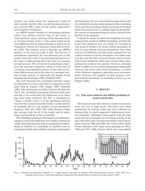
232Clim Res 43: 229–239, 2010models, was tested using the significance levels ofeach variable and the effect on the Bayesian informationcriterion (BIC) value for the model, using backwardstepwise techniques.An ARIMA model consists of a forecasting equationwhich may include previous lags in the series, or‘autoregressive’ terms, and lags of the forecast errors,or ‘moving average’ terms. A time series which needsto be differenced to be made stationary is said to be an‘integrated’ version of a stationary series (Box & Jenkins1976). The notation used to describe an ARIMAmodel is of the form (p d q)(P D Q)S. The first set ofparentheses represents the non-seasonal part of themodel, with p the order of an autoregressive process, dthe order of differencing and q the order of a movingaverage process. The second set of parentheses representsthe seasonal component, where P is the order ofa seasonal autoregressive process, D the order of seasonaldifferencing and Q the order of a seasonal movingaverage process. S represents the length of theseasonal period (Diggle 1990, Chatfield 1997).The ACF measures the correlation between valuesat each point in a series and values at lags prior to thatpoint (Box & Jenkins 1976, Diggle 1990, Chatfield1997). This information is further used to calculate thePACF, the correlation remaining between each pointand lag in the series after the influences of all closerlags have been removed. The BIC is calculated as–2ln(L) + ln(n)k, where L is the likelihood functionbased on the residuals from the model, n is the numberof residuals and k is the number of free parameters(Schwarz 1978, Wei 1990). This value therefore takesinto account both the fit of the model and its parsimony,and should be as low as possible.The modelling techniques developed were phenomenological,in the sense that they were neither constrainedwithin a theoretical framework nor analysed mechanisticallyin relation to a multitude of variables such asvegetation density and condition, soil types, temperatureand hydrology. We were interested in seeing what couldbe concluded from time series analyses of the locust dataalone and then in testing whether inclusion of the mainfactor in locust survival, i.e. rainfall, improved the predictivepower of phenomenological models derived fromthe time series analyses.It should be borne in mind that sampling error mayconfound the results of ARIMA modelling, and that thelocust data analysed here are based on coverage ofvast areas of territory by locust control personnel, aswell as from reports of locust infestations from othersources. Furthermore, the time series analysed are nota direct measure of locust abundance, but rather indicatethe area that they covered during a given month.Both factors should be taken into account when interpretingthe results of the analysis. However, althoughthere is unlikely to be a strict proportional relationshipbetween this series and actual abundance, a reviewof the literature suggests a generally good correspondencebetween the numbers of grid squares occupiedand the abundance of swarming locusts (e.g. seePedgley 1981).3. RESULTS3.1. Time series analyses and ARIMA modelling oflocust swarms dataThe locust swarms data showed a series of increasesfrom very low to high levels. The latter were oftenmaintained for several years and were followed bydeclines (Fig. 2), which suggested a high degree of serialcorrelation. Although it may appear from the timeseries that locust plagues are becoming a thing of thepast, this series does not show the plague which developedbetween 1988 and 1989, the recent (2003–2005)locust outbreak or the major locust upsurges in 1992–1994 and 1997–1998, data for which were unavailableNo. of squares500400300200100Grid squares1009080706050403020100J F M A M J J A S O N DMonth030 33 36 39 42 45 48 51 54 57 60 63 66 69 72 75 78 81 84 87YearFig. 2. Schistocerca gregaria. Number of 1° grid squares reported as infested with desert locust swarms, 1930–1987, as amonthly time series I, and mean numbers summarised by month (inset, in which error bars show ±2 SE)
Page 3: 230Clim Res 43: 229-239, 2010Desert
Page 7 and 8: 234Clim Res 43: 229-239, 2010Table
Page 9 and 10: 236Clim Res 43: 229-239, 2010Grid s
Page 11: 238Clim Res 43: 229-239, 2010that r

Desert locust populations, rainfall and climate change: insights from ...

Create successful ePaper yourself

Delete template?

Save as template?