Desert locust populations, rainfall and climate change: insights from ...

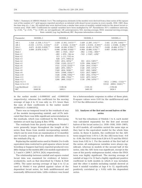
234Clim Res 43: 229–239, 2010Table 1. Summary of ARIMA Models 1 to 4. The endogenous elements in the models were derived from a time series of the squareroot of the number of 1° grid squares reported anywhere as infested with desert locust swarms in every month, 1930–1987; thus,the time step (t) = 1 mo. All rainfall data were derived from a similar time series of monthly rainfall totals for the desert locust recessionarea, 1928–1987. Coefficients for rainfall variables have been multiplied by 10 8 . Parentheses: 95% confidence intervals,*p < 0.05, **p < 0.01, ***p < 0.001, ns: not significant. AR: autoregressive; MA: moving average; SMA: seasonal moving average;Rain: rainfall; Log: log likelihood; BIC: Bayesian information criterionParameter MODEL 1 MODEL 2 MODEL 3 MODEL 4AR 1 1.524 (1.338, 1.711)*** 1.459 (1.301, 1.617)*** 1.449 (1.287, 1.61)*** 1.441 (1.279, 1.603)***AR 2 –0.535 (–0.715, –0.355)** –0.47 (–0.622, –0.318)** –0.459 (–0.616, –0.303)** –0.452 (–0.608, –0.296)**MA 1 0.671 (0.503, 0.839)*** 0.646 (0.506, 0.785)*** 0.634 (0.491, 0.778)*** 0.628 (0.484, 0.771)***SMA 1 0.899 (0.878, 0.92)*** 0.906 (0.884, 0.928)*** 0.908 (0.886, 0.93)*** 0.907 (0.885, 0.928)***Rain t –683 (–1025, –341)* –862 (–1164, –560)**Rain t-1 –482 (–870, –94) ns –743 (–1047, –439)*Rain t-2 313 (–111, 737) nsRain t-3 628 (171, 1085) nsRain t-4 1393 (912, 1874)** 951 (615, 1287)**Rain t-5 1708 (1205, 2211)*** 1279 (904, 1654)***Rain t-6 1721 (1210, 2232)*** 1320 (910, 1730)**Rain t-7 1483 (975, 1991)** 1140 (707, 1573)**Rain t-8 1340 (854, 1826)** 1037 (605, 1469)*Rain t-9 1470 (1006, 1934)** 1253 (817, 1689)**Rain t-10 1526 (1096, 1956)*** 1363 (952, 1774)***Rain t-11 1372 (982, 1762)*** 1253 (873, 1633)**Rain t-12 1206 (860, 1552)*** 1130 (790, 1470)***Rain t to t-1 –1612 (–2092, –1132)***Rain t-4 to t-12 10152 (8063, 12241)***Log likelihood –1211.12 –1190.56 –1191.55 –1192.66BIC 2448.36 2492.1 2481.03 2424.5in the earlier model (–0.0000161 and –0.0000160respectively), whereas the coefficient for the movingaverage of lags 4 to 12 was only ca. 6% lower thanthe sum of their coefficients in the earlier model(0.0001013 < 0.0001072).There was no temporal trend in the residuals of anyof the models incorporating rainfall, and ACFs indicatedthat there was little significant autocorrelation inthe residuals, which was confirmed by the Box-Ljungstatistics at each lag (Ljung & Box 1978).The residuals from the purely endogenous Model 1were generally larger throughout the length of theseries than those from models incorporating rainfall,which can be seen from an examination of 12-monthlyand 6-yearly averages of the absolute differences inthe residuals (Fig. 4).Replacing the rainfall series used in Models 2 to 4 withequivalent data restricted to grid squares where locustbreeding or hoppers had been reported produced verylittle change in the models (BICs for models equivalent to2, 3 and 4 = 2490.7, 2479.9, 2424, respectively).The relationship between rainfall and square-rootedlocust data was examined for evidence of heteroscedasticity,such as that described by Cheke & Holt(1993). The same moving average of lags 4 to 12 asused in Model 4 was plotted against values of thedependent locust series, for both undifferenced andseasonally differenced data. Little evidence was foundfor a heteroscedastic response in either of these plots.R-square values were 0.05 for the undifferenced and0.17 for the differenced series.3.3. Analyses of the first and second halves of theseriesTo test the robustness of Models 1 to 4, each modelwas calculated separately for the first and secondhalves of the locust series (i.e. 1930–1958, 1959–1987).In all 8 models, all variables carried the same sign asthey had in the equivalent model for the whole timeseries. In these 8 models, the coefficient for the AR1term ranged from 1.05 to 1.59, the AR2 term from –0.6to –0.06, the MA1 term from 0.26 to 0.73 and the SMA1term from 0.82 to 1. For the models of the first half ofthe series, all endogenous variables were always significant,whereas in models of the second half of theseries, only the AR1 term was significant, except in thecase of the purely endogenous model, where the SMAterm was highly significant. The moving average ofrainfall at lags 4 to 12 had a highly significant positivecoefficient in both models in which it was included,and the other 4 models including rainfall showed atleast 4 rainfall variables at lags 4 to 12, significantlypositively correlated (p < 0.05) with the dependentseries.