Desert locust populations, rainfall and climate change: insights from ...

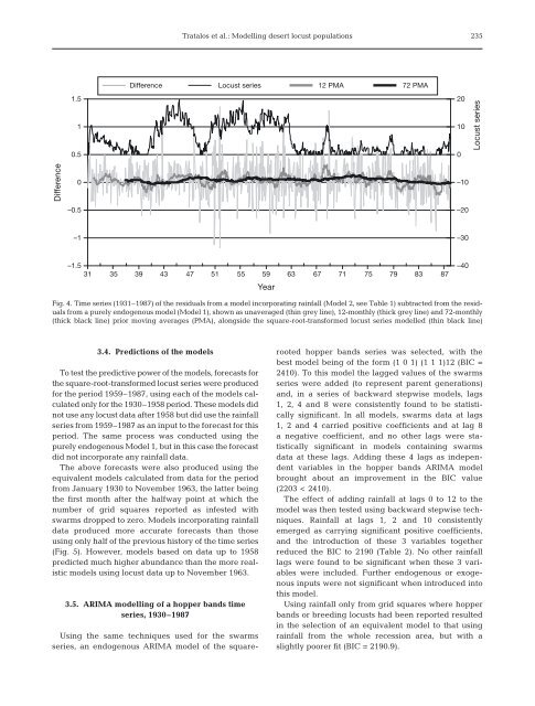
Tratalos et al.: Modelling desert locust populations235Difference Locust series 12 PMA 72 PMADifference1.510.50–0.520100–10–20Locust series–1–30–1.531 35 39 43 47 51 55 59Year63 67 71 75 79 83 87–40Fig. 4. Time series (1931–1987) of the residuals from a model incorporating rainfall (Model 2, see Table 1) subtracted from the residualsfrom a purely endogenous model (Model 1), shown as unaveraged (thin grey line), 12-monthly (thick grey line) and 72-monthly(thick black line) prior moving averages (PMA), alongside the square-root-transformed locust series modelled (thin black line)3.4. Predictions of the modelsTo test the predictive power of the models, forecasts forthe square-root-transformed locust series were producedfor the period 1959–1987, using each of the models calculatedonly for the 1930–1958 period. These models didnot use any locust data after 1958 but did use the rainfallseries from 1959–1987 as an input to the forecast for thisperiod. The same process was conducted using thepurely endogenous Model 1, but in this case the forecastdid not incorporate any rainfall data.The above forecasts were also produced using theequivalent models calculated from data for the periodfrom January 1930 to November 1963, the latter beingthe first month after the halfway point at which thenumber of grid squares reported as infested withswarms dropped to zero. Models incorporating rainfalldata produced more accurate forecasts than thoseusing only half of the previous history of the time series(Fig. 5). However, models based on data up to 1958predicted much higher abundance than the more realisticmodels using locust data up to November 1963.3.5. ARIMA modelling of a hopper bands timeseries, 1930–1987Using the same techniques used for the swarmsseries, an endogenous ARIMA model of the squarerootedhopper bands series was selected, with thebest model being of the form (1 0 1) (1 1 1)12 (BIC =2410). To this model the lagged values of the swarmsseries were added (to represent parent generations)and, in a series of backward stepwise models, lags1, 2, 4 and 8 were consistently found to be statisticallysignificant. In all models, swarms data at lags1, 2 and 4 carried positive coefficients and at lag 8a negative coefficient, and no other lags were statisticallysignificant in models containing swarmsdata at these lags. Adding these 4 lags as independentvariables in the hopper bands ARIMA modelbrought about an improvement in the BIC value(2203 < 2410).The effect of adding rainfall at lags 0 to 12 to themodel was then tested using backward stepwise techniques.Rainfall at lags 1, 2 and 10 consistentlyemerged as carrying significant positive coefficients,and the introduction of these 3 variables togetherreduced the BIC to 2190 (Table 2). No other rainfalllags were found to be significant when these 3 variableswere included. Further endogenous or exogenousinputs were not significant when introduced intothis model.Using rainfall only from grid squares where hopperbands or breeding locusts had been reported resultedin the selection of an equivalent model to that usingrainfall from the whole recession area, but with aslightly poorer fit (BIC = 2190.9).