Desert locust populations, rainfall and climate change: insights from ...

More documents

Recommendations

Info

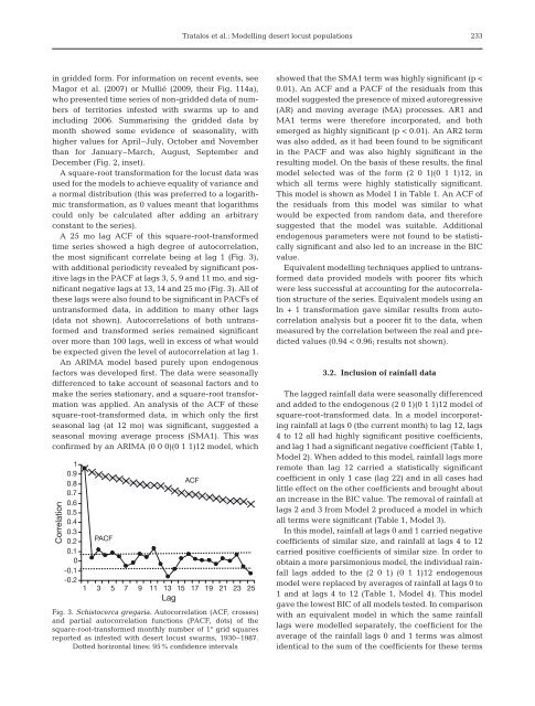
Tratalos et al.: Modelling desert locust populations233in gridded form. For information on recent events, seeMagor et al. (2007) or Mullié (2009, their Fig. 114a),who presented time series of non-gridded data of numbersof territories infested with swarms up to andincluding 2006. Summarising the gridded data bymonth showed some evidence of seasonality, withhigher values for April–July, October and Novemberthan for January–March, August, September andDecember (Fig. 2, inset).A square-root transformation for the locust data wasused for the models to achieve equality of variance anda normal distribution (this was preferred to a logarithmictransformation, as 0 values meant that logarithmscould only be calculated after adding an arbitraryconstant to the series).A 25 mo lag ACF of this square-root-transformedtime series showed a high degree of autocorrelation,the most significant correlate being at lag 1 (Fig. 3),with additional periodicity revealed by significant positivelags in the PACF at lags 3, 5, 9 and 11 mo, and significantnegative lags at 13, 14 and 25 mo (Fig. 3). All ofthese lags were also found to be significant in PACFs ofuntransformed data, in addition to many other lags(data not shown). Autocorrelations of both untransformedand transformed series remained significantover more than 100 lags, well in excess of what wouldbe expected given the level of autocorrelation at lag 1.An ARIMA model based purely upon endogenousfactors was developed first. The data were seasonallydifferenced to take account of seasonal factors and tomake the series stationary, and a square-root transformationwas applied. An analysis of the ACF of thesesquare-root-transformed data, in which only the firstseasonal lag (at 12 mo) was significant, suggested aseasonal moving average process (SMA1). This wasconfirmed by an ARIMA (0 0 0)(0 1 1)12 model, whichCorrelation10.90.80.70.60.50.40.30.20.10-0.1-0.2PACFACF1 3 5 7 9 11 13 15 17 19 21 23 25LagFig. 3. Schistocerca gregaria. Autocorrelation (ACF, crosses)and partial autocorrelation functions (PACF, dots) of thesquare-root-transformed monthly number of 1° grid squaresreported as infested with desert locust swarms, 1930–1987.Dotted horizontal lines: 95% confidence intervalsshowed that the SMA1 term was highly significant (p
234Clim Res 43: 229–239, 2010Table 1. Summary of ARIMA Models 1 to 4. The endogenous elements in the models were derived from a time series of the squareroot of the number of 1° grid squares reported anywhere as infested with desert locust swarms in every month, 1930–1987; thus,the time step (t) = 1 mo. All rainfall data were derived from a similar time series of monthly rainfall totals for the desert locust recessionarea, 1928–1987. Coefficients for rainfall variables have been multiplied by 10 8 . Parentheses: 95% confidence intervals,*p < 0.05, **p < 0.01, ***p < 0.001, ns: not significant. AR: autoregressive; MA: moving average; SMA: seasonal moving average;Rain: rainfall; Log: log likelihood; BIC: Bayesian information criterionParameter MODEL 1 MODEL 2 MODEL 3 MODEL 4AR 1 1.524 (1.338, 1.711)*** 1.459 (1.301, 1.617)*** 1.449 (1.287, 1.61)*** 1.441 (1.279, 1.603)***AR 2 –0.535 (–0.715, –0.355)** –0.47 (–0.622, –0.318)** –0.459 (–0.616, –0.303)** –0.452 (–0.608, –0.296)**MA 1 0.671 (0.503, 0.839)*** 0.646 (0.506, 0.785)*** 0.634 (0.491, 0.778)*** 0.628 (0.484, 0.771)***SMA 1 0.899 (0.878, 0.92)*** 0.906 (0.884, 0.928)*** 0.908 (0.886, 0.93)*** 0.907 (0.885, 0.928)***Rain t –683 (–1025, –341)* –862 (–1164, –560)**Rain t-1 –482 (–870, –94) ns –743 (–1047, –439)*Rain t-2 313 (–111, 737) nsRain t-3 628 (171, 1085) nsRain t-4 1393 (912, 1874)** 951 (615, 1287)**Rain t-5 1708 (1205, 2211)*** 1279 (904, 1654)***Rain t-6 1721 (1210, 2232)*** 1320 (910, 1730)**Rain t-7 1483 (975, 1991)** 1140 (707, 1573)**Rain t-8 1340 (854, 1826)** 1037 (605, 1469)*Rain t-9 1470 (1006, 1934)** 1253 (817, 1689)**Rain t-10 1526 (1096, 1956)*** 1363 (952, 1774)***Rain t-11 1372 (982, 1762)*** 1253 (873, 1633)**Rain t-12 1206 (860, 1552)*** 1130 (790, 1470)***Rain t to t-1 –1612 (–2092, –1132)***Rain t-4 to t-12 10152 (8063, 12241)***Log likelihood –1211.12 –1190.56 –1191.55 –1192.66BIC 2448.36 2492.1 2481.03 2424.5in the earlier model (–0.0000161 and –0.0000160respectively), whereas the coefficient for the movingaverage of lags 4 to 12 was only ca. 6% lower thanthe sum of their coefficients in the earlier model(0.0001013 < 0.0001072).There was no temporal trend in the residuals of anyof the models incorporating rainfall, and ACFs indicatedthat there was little significant autocorrelation inthe residuals, which was confirmed by the Box-Ljungstatistics at each lag (Ljung & Box 1978).The residuals from the purely endogenous Model 1were generally larger throughout the length of theseries than those from models incorporating rainfall,which can be seen from an examination of 12-monthlyand 6-yearly averages of the absolute differences inthe residuals (Fig. 4).Replacing the rainfall series used in Models 2 to 4 withequivalent data restricted to grid squares where locustbreeding or hoppers had been reported produced verylittle change in the models (BICs for models equivalent to2, 3 and 4 = 2490.7, 2479.9, 2424, respectively).The relationship between rainfall and square-rootedlocust data was examined for evidence of heteroscedasticity,such as that described by Cheke & Holt(1993). The same moving average of lags 4 to 12 asused in Model 4 was plotted against values of thedependent locust series, for both undifferenced andseasonally differenced data. Little evidence was foundfor a heteroscedastic response in either of these plots.R-square values were 0.05 for the undifferenced and0.17 for the differenced series.3.3. Analyses of the first and second halves of theseriesTo test the robustness of Models 1 to 4, each modelwas calculated separately for the first and secondhalves of the locust series (i.e. 1930–1958, 1959–1987).In all 8 models, all variables carried the same sign asthey had in the equivalent model for the whole timeseries. In these 8 models, the coefficient for the AR1term ranged from 1.05 to 1.59, the AR2 term from –0.6to –0.06, the MA1 term from 0.26 to 0.73 and the SMA1term from 0.82 to 1. For the models of the first half ofthe series, all endogenous variables were always significant,whereas in models of the second half of theseries, only the AR1 term was significant, except in thecase of the purely endogenous model, where the SMAterm was highly significant. The moving average ofrainfall at lags 4 to 12 had a highly significant positivecoefficient in both models in which it was included,and the other 4 models including rainfall showed atleast 4 rainfall variables at lags 4 to 12, significantlypositively correlated (p < 0.05) with the dependentseries.
Page 3 and 4: 230Clim Res 43: 229-239, 2010Desert
Page 5: 232Clim Res 43: 229-239, 2010models
Page 9 and 10: 236Clim Res 43: 229-239, 2010Grid s
Page 11: 238Clim Res 43: 229-239, 2010that r

Desert locust populations, rainfall and climate change: insights from ...

Create successful ePaper yourself

Delete template?

Save as template?