Desert locust populations, rainfall and climate change: insights from ...

More documents

Recommendations

Info

Tratalos et al.: Modelling desert locust populations235Difference Locust series 12 PMA 72 PMADifference1.510.50–0.520100–10–20Locust series–1–30–1.531 35 39 43 47 51 55 59Year63 67 71 75 79 83 87–40Fig. 4. Time series (1931–1987) of the residuals from a model incorporating rainfall (Model 2, see Table 1) subtracted from the residualsfrom a purely endogenous model (Model 1), shown as unaveraged (thin grey line), 12-monthly (thick grey line) and 72-monthly(thick black line) prior moving averages (PMA), alongside the square-root-transformed locust series modelled (thin black line)3.4. Predictions of the modelsTo test the predictive power of the models, forecasts forthe square-root-transformed locust series were producedfor the period 1959–1987, using each of the models calculatedonly for the 1930–1958 period. These models didnot use any locust data after 1958 but did use the rainfallseries from 1959–1987 as an input to the forecast for thisperiod. The same process was conducted using thepurely endogenous Model 1, but in this case the forecastdid not incorporate any rainfall data.The above forecasts were also produced using theequivalent models calculated from data for the periodfrom January 1930 to November 1963, the latter beingthe first month after the halfway point at which thenumber of grid squares reported as infested withswarms dropped to zero. Models incorporating rainfalldata produced more accurate forecasts than thoseusing only half of the previous history of the time series(Fig. 5). However, models based on data up to 1958predicted much higher abundance than the more realisticmodels using locust data up to November 1963.3.5. ARIMA modelling of a hopper bands timeseries, 1930–1987Using the same techniques used for the swarmsseries, an endogenous ARIMA model of the squarerootedhopper bands series was selected, with thebest model being of the form (1 0 1) (1 1 1)12 (BIC =2410). To this model the lagged values of the swarmsseries were added (to represent parent generations)and, in a series of backward stepwise models, lags1, 2, 4 and 8 were consistently found to be statisticallysignificant. In all models, swarms data at lags1, 2 and 4 carried positive coefficients and at lag 8a negative coefficient, and no other lags were statisticallysignificant in models containing swarmsdata at these lags. Adding these 4 lags as independentvariables in the hopper bands ARIMA modelbrought about an improvement in the BIC value(2203 < 2410).The effect of adding rainfall at lags 0 to 12 to themodel was then tested using backward stepwise techniques.Rainfall at lags 1, 2 and 10 consistentlyemerged as carrying significant positive coefficients,and the introduction of these 3 variables togetherreduced the BIC to 2190 (Table 2). No other rainfalllags were found to be significant when these 3 variableswere included. Further endogenous or exogenousinputs were not significant when introduced intothis model.Using rainfall only from grid squares where hopperbands or breeding locusts had been reported resultedin the selection of an equivalent model to that usingrainfall from the whole recession area, but with aslightly poorer fit (BIC = 2190.9).
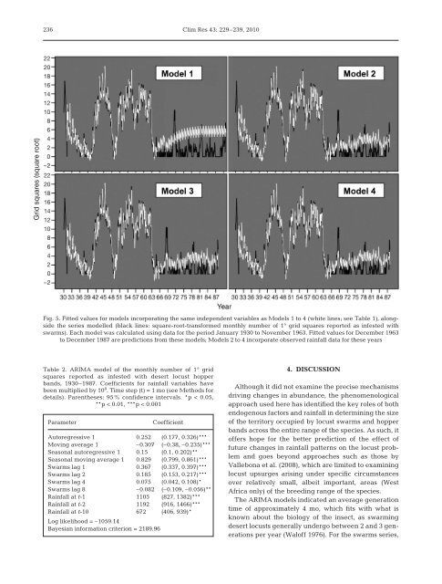
236Clim Res 43: 229–239, 2010Grid squares (square root)2220181614121086420–22220181614121086420–2Fig. 5. Fitted values for models incorporating the same independent variables as Models 1 to 4 (white lines; see Table 1), alongsidethe series modelled (black lines: square-root-transformed monthly number of 1° grid squares reported as infested withswarms). Each model was calculated using data for the period January 1930 to November 1963. Fitted values for December 1963to December 1987 are predictions from these models; Models 2 to 4 incorporate observed rainfall data for these yearsTable 2. ARIMA model of the monthly number of 1° gridsquares reported as infested with desert locust hopperbands, 1930–1987. Coefficients for rainfall variables havebeen multiplied by 10 8 . Time step (t) = 1 mo (see Methods fordetails). Parentheses: 95% confidence intervals. *p < 0.05,**p < 0.01, ***p < 0.001ParameterCoefficientAutoregressive 1 0.252 (0.177, 0.326)***Moving average 1 –0.307 (–0.38, –0.235)***Seasonal autoregressive 1 0.15 (0.1, 0.202)**Seasonal moving average 1 0.829 (0.799, 0.861)***Swarms lag 1 0.367 (0.337, 0.397)***Swarms lag 2 0.185 (0.153, 0.217)***Swarms lag 4 0.075 (0.042, 0.108)*Swarms lag 8 –0.082 (–0.109, –0.056)**Rainfall at t-1 1105 (827, 1382)***Rainfall at t-2 1192 (916, 1466)***Rainfall at t-10 672 (406, 939)*Log likelihood = –1059.14Bayesian information criterion = 2189.964. DISCUSSIONAlthough it did not examine the precise mechanismsdriving changes in abundance, the phenomenologicalapproach used here has identified the key roles of bothendogenous factors and rainfall in determining the sizeof the territory occupied by locust swarms and hopperbands across the entire range of the species. As such, itoffers hope for the better prediction of the effect offuture changes in rainfall patterns on the locust problemand goes beyond approaches such as those byVallebona et al. (2008), which are limited to examininglocust upsurges arising under specific circumstancesover relatively small, albeit important, areas (WestAfrica only) of the breeding range of the species.The ARIMA models indicated an average generationtime of approximately 4 mo, which fits with what isknown about the biology of the insect, as swarmingdesert locusts generally undergo between 2 and 3 generationsper year (Waloff 1976). For the swarms series,
Page 3 and 4: 230Clim Res 43: 229-239, 2010Desert
Page 5 and 6: 232Clim Res 43: 229-239, 2010models
Page 7: 234Clim Res 43: 229-239, 2010Table
Page 11: 238Clim Res 43: 229-239, 2010that r

Desert locust populations, rainfall and climate change: insights from ...

You also want an ePaper? Increase the reach of your titles

Delete template?

Save as template?