Affluence and Food: A Simple Way to Infer Incomes - The University ...

ECONOMICSAFFLUENCE AND FOODA Simple Way to Infer IncomesbyKenneth W ClementsBusiness SchoolThe University of Western AustraliaandDongling ChenShanghai Municipal AuthorityDISCUSSION PAPER 09.08

AFFLUENCE AND FOODA Simple Way to Infer Incomes 1byKenneth W ClementsBusiness SchoolThe University of Western AustraliaandDongling ChenShanghai Municipal AuthorityAbstractAccurate and timely measures of cross-country real incomes are still a rarity. As the share ofexpenditure devoted to food is readily available, we use of Engel’s law in reciprocal form to measureaffluence. Analysis of real income data for the OECD countries indicates that this approach is viable.To recognise the role of uncertainty in the analysis, we present the results in the form of stochasticcross-country income comparisons.1 We would like to acknowledge the comments of Grace Gao and the excellent research assistance of Ze Min Hu, Shi Pei Seah andJiawei Si. This research was supported in part by the ARC.

1. IntroductionEconomists’ fascination with international income differences must go back to at least 1776 withAdam Smith’s The Wealth of Nations. The most popular approach to measuring incomes in differentcountries is to use the purchasing-power-parity based estimates of the Penn Table. As market exchange ratesare volatile, and are known to reflect the prices of nontraded goods (especially services) less than adequately,the PPP method is a substantial improvement over older approaches that make currency conversions on thebasis of market exchange rates. However, the disadvantage of PPP is that as numerous matched goods andservices have to be priced in many countries, it is demanding in its data requirements, so that PPP estimatescan be subject to long publication delays. This paper investigates a short-cut method of measuring realincomes across countries.Engel’s law states that food has an income elasticity of less than unity, or equivalently, the share offood in the consumption basket declines with income. We use Engel’s law in reciprocal form by inferringincome from the value of the food share. Such an approach is consistent with Engel (1857, pp. 28-29) whowrites “The poorer a family, the greater the proportion of its total expenditure that must be devoted to theprovision of food”, and then goes on to argue that the richer a country, the smaller the food share (Stigler,1954). This approach has several advantages: First, as the food share is dimensionless, it can be comparedacross time, regions and countries, without any adjustment for differing currency values. Second, the foodshare is objective, not subject to great controversy and readily available for many time periods in a largenumber of countries. Third, the link between the food share and income as enshrined in Engel’s law is wellestablished and arguably the most widely-accepted empirical regularity in all economics. Finally, as theapproach uses just one share and two parameters to make inferences regarding incomes, it is attractive in itssimplicity. We analyse jointly the determinants of all elements in the consumption basket and embed Engel’slaw in a system-wide demand model, thereby allowing for the dependence of food share on relative prices (inaddition to income). The food share, adjusted for differing relative price structures across countries, is thenused to infer income.While the basic idea of employing the food share as an inverse measure of welfare has been used byothers (see, e. g., Orshansky, 1965, 1969, Van Praag et al., 1982, Rao, 1981), it seems that the approach ofincluding food in a microeconomic demand model, and then using the price-adjusted share as the basis forinferring income, has been relatively unexplored, especially in a cross-country context. Chua (2003) made apreliminary investigation of estimating “true income” in different countries from information on the foodshare, but did not allow for international differences in relative prices. For related studies that deal with theCPI bias and economic performance in the US, see Costa (2001), Hamilton (2001) and Nakamura (1996).1

n(1) qˆ= η Mˆ+ ∑ η ′ p ˆ ,i i ij jj=1where ηiis the income elasticity of demand for i and η ′ijis the ( i, j ) thuncompensated price elasticity. If wedefine the change in the cost of living index as a budget-share weighted-average of the n price changes,Pˆ= w pˆ, then the change in real income is the excess of the change in money income change over thisn∑ j=1jjindex, Q ˆ = M ˆ − P ˆ , and the Slutsky demand equation takes the formi i ij jj=1( ˆ ˆ)n(2) qˆ= η Qˆ+ ∑ η p − P ,whereη is the ( i, j ) thcompensated price elasticity. In deriving this equation (2) from (1), we have used (i)ijnthe Slutsky decomposition η ′ij= ηij − wjη i, and (ii) demand homogeneity, according to which ∑ j = 1 ηij= 0.ŵ = pˆ + qˆ − M = pˆ − P + qˆ− Qˆ. Combining this with equation (2) then yieldsNext, we note that ˆ(ˆ)i i i i i( ) ˆ ∑n( ˆ ˆ) ( ˆ ˆ)(3) wˆ= η − 1 Q + η p − P + p − P .i i ij j ij=1If the n commodities are broad aggregates, it would be likely that there would only be limitedsubstitutability between them. We thus take the utility function to be of the preference independentnform, u ( q ,…,q ) = ∑ i = 1u ( q ) , with u ( )1 n i iii the sub-utility function for good i, so that the marginal utility ofi depends only on own consumption. This form of tastes implies that as an approximation, own-priceelasticties are proportional to income elasticities and cross-price elasticities are zero,(4) η ≈ φη , i = 1, …, n, η ≈ 0, i, j = 1, …, n,i ≠ j,ii i ijwhere φ is the reciprocal of the income elasticity of the marginal utility of income (the “income flexibility”for short). Equations (3) and (4) then imply( ) ˆ ( )( ˆ ˆ)(5) wˆ≈ η − 1 Q + φη + 1 p − P ,i i i iwhich shows the dependence of the budget share on income and the relative price of the good. The twoparameters in equation (5) are the income elasticity and the income flexibility.3. Income and FoodOn the basis of the budget shares, in most countries food is the most important single commodity.Thus, in what follows we concentrate on this commodity. In this section, we analyse the relationship3

etween food consumption and income, and defer a discussion of the role of its relative price until the nextsection.We apply equation (5) to i = food and for simplicity, subsequently omit the commodity subscript.When the relative price of food is constant, this equation impliesshare of food is ( pq)dw ≈ β Qˆ, with β = w ( η − 1). The marginal∂ ∂ M , which answers the question, if income rises by one dollar, what fraction of thisis spent on food? As wη = ∂ ( pq)∂ M , it follows that the coefficient β is the excess of the marginal shareover the corresponding budget share w . Using ˆx d( log x)food consumption and income in countries a and b is⎛ Q ⎞− = β ⎜ ⎟ .⎝ ⎠a(6)a bw w log Qb= , the above suggests a convenient way to relateTable 1 gives for 42 OECD countries in 2002 real per capita total consumption, which we interpret asQ, and the food budget share. 4 As can be seen, on the basis of Q, Luxembourg is the richest country andTurkey the poorest, with a ratio of 30, 258 4,882 ≈ 6 , while the food budget shares range from less than 10percent to about 30 percent. The budget share of each country can be systematically compared to that of allothers via 42× 42 skewed symmetric matrix⎡⎣wab− w ⎤⎦ . The upper triangle of this matrix is given in Table2, where countries are ordered in terms of decreasing affluence in the rows and increasing affluence in thecolumns. Thus, for example, moving from left to right along the first row, we compare the food budgetshare of Luxembourg with poorer countries that become successively less poor: The share for Turkey is 17points above Luxembourg’s, Macedonia’s 22 above, etc. As the diagonal elements of this table would be allzero, these elements are suppressed. But as we move further away from where the diagonal would havebeen, in a north-westerly direction, countries differ more on the income scale and the budget shares differ bymore. With only a few exceptions, for each pairwise comparison, the share in the poorer country is greaterthan that in the richer country, which is a reflection of Engel’s law.Table 3 gives the corresponding matrix comparisons of incomes, which for short we write as( )ab a b∆ log Q = log Q Q . Table 4 contains the ratiosabab∆w∆ log Q , whereab a b∆ w = w − w . These ratioscan be interpreted as “readings” on the coefficient β in equation (6). Figure 1 shows that while there are afew outliers (associated with near zeros in the denominators for countries having very similar incomes), thedistribution has a reasonable well defined median of about -0.13. This result is confirmed by thecorresponding scatter of Figure 2. When β = − 0.13 , a country that is 50 percent richer than another has a4 The data are from OECD (2004). For details, see the Appendix.4

food budget share about 5 percentage points lower. If we only used information on the food share, we couldlog Q 1 wabemploy this relationship in reciprocal form whereby ( )ab∆ = β ∆ to make inferences regardingincome differences. In Section 5 we extend this basic relationship to allow for the role of differences inrelative prices, and demonstrate the importance of allowing for the impact of this additional factor.Before concluding this section, it is worthwhile noting that by integration, equation (6) is consistentwith the Working (1943)-Leser (1963) Engel curve, w= α + β log Q , where α is a constant. Figure 3 revealsthat this model fits the OECD data quite well, and the least-squares estimate of the slope coefficient β isclose to the above-value of -0.13.4. Modelling the Consumption BasketAs indicated by equation (5), the change in the budget share of good i is related to the change inincome and under the assumption of preference independence, the change in the relative price of the good.The parameters in this relationship are the income elasticity and the income flexibility. To efficientlyestimate these parameters, we need to consider the demand for all n goods simultaneously by jointlymodeling the determinants of the consumption basket. There are a number of alternative models that couldbe used for this purpose including the linear expenditure system, the almost ideal demand model, thetranslog, etc. We choose the Florida model (Theil et al., 1989) as it is probably the most extensively appliedand assessed in a cross-country context.In this section, we reinstate the commodity subscript i = 1,…,n, and denote countries by c = 1,…,C.The Florida model is based on Working’s model,(7) w log Qwherecci= αi+ βi,n nαiand βiare coefficients satisfying ∑i= 1α = 1, ∑i=1β = 0. If we denote the logarithm of real incomeiiin country c byqcc= log Q , it can be easily shown that model (7) implies that the marginal share of good itakes the formαi+ βi q∗c , where∗ccq 1 qC cmeasured by geometric means, ( )cii= + . The Florida model supposes that (7) holds at world prices, aslog p = 1 C ∑ log pc⎡c nc c c pp ⎤ic j(8) wi=αi+βiq + ( αi+βiq ) ⎢log -∑( αj+β jq ) log ⎥⎢⎣pij=1pj ⎥⎦c=1c⎡c nc pp ⎤∗i∗cj+ φ( αi+βiq ) ⎢log -∑(αj+β jq ) log ⎥⎢⎣pij=1pj⎥⎦+ε ,i. The i th equation of the model takes the form5

where φ is the income flexibility (as before) andcεiis a zero-mean disturbance term, drawn from amultivariate normal distribution with a constant covariance matrix. The second term on the right-hand sideof this equation,cβiq , deals with the role of real income on the budget share of good i, while the first termin square brackets is the relative price of the good, compared to the world relative price. When the relativeprice changes, the budget share changes even when the corresponding quantity demanded is unchanged; thisnciceffect is measured by the term ( i i ) ⎢ ∑ ( j j )cc⎡ pp ⎤jα +β q log - α +β q log ⎥ . The second line of equation (8) deals⎢⎣pij=1pj⎥⎦with the substitution effect of a change in the relative price of the good; the weights employed in this relativeprice are marginal shares,α +β q ∗jjc, whereas in the first line of the equation they are budget shares,cαj+β jq .The final thing to note about the Florida model is that it holds under preference independence, so it isconsistent with the analysis of Section 2 above.We estimate model (8) using the maximum likelihood (ML) procedure set out in Theil et al. (1989)with data from the OECD (2004) for n = 12 goods listed in Table 5 and the C = 42 countries listed in Table1. The results are given in columns 2-5 of Table 5. The largest estimate of βi(in absolute value) is for foodat -0.10, a value that is highly significant. That this value is about 25 percent lower than the estimate of thissame coefficient discussed in the previous section indicates the importance of controlling for differences inthe relative price of food across countries. An examination of the data reveals that this relative price tends tofall with real income per capita, so that omitting it has the effect of biasing upwards the estimate offood.6βiforTo assess the quality of the estimates, we conduct a Monte Carlo experiment that involves thefollowing steps. First, we write model (8) for i = 1,…,12 as( θ)(9) w c = f X c , θ + εc ,wherecw andεcε are vectors of budget shares and disturbances for country c,cX is a matrix of the observedvalues of the independent variables and θ is a vector of parameters. We simulate the budget vector forcountry c from equation (9) by (i) drawingεcfrom a normal distribution with mean vector zero andcovariance matrix equal to its data-based ML estimate; (ii) using for θ its data-based estimate; and (iii)using the observed values ofsimulated vector of budget shares, wcX . Repeating this for each of the 42 countries leads to 42 values of thec(s), c =1,…,42, which are used together with the observed values of theindependent variables to reestimate the model by the same ML procedure. Second, we repeat the procedure1,000 times to yield 1,000 simulated values of the vector of estimated parameters, θ (s) ,s = 1, …,1,000.

Columns 6-11 of Table 5 summarise the results in the form of the mean, RMSE and RMASE for eachparameter. As can be seen, all estimates are unbiased, while the asymptotic standard errors tend to understatethe sampling variability of the estimates, but not by a huge amount.5. Simulating IncomeIn this section we draw inferences on cross-country incomes from the behavour of the food budgetshare after controlling the influence of the relative price. As before, we concentrate exclusively on food anddrop the commodity subscript.We return to equation (5) and write it as( φη + 1)( pˆ− P ˆ )ˆ ŵ(5′) Q = −,η −1 η −1where ˆQ is the change in income, ŵ the change in the food budget share, η is the income elasticity of food,φ is the income flexibility,ˆp− Pˆis the change in the relative price of food, and where we have ignored theapproximation error. This equation says that the change in income is equal to the difference between a terminvolving the change in the food share and a term that adjusts for the change in the relative price of food. Toapply equation (5′)to countries a and b, we could express it asa bab a b a b( w ) ( φη + 1) ⎡log ( p p ) − log ( P P )a⎛ Q ⎞ log w⎤(5′′) log⎣ ⎦⎜,b ⎟ = −ab ab⎝ Q ⎠ η −1 η −11η = η + η is the average of the income elasticity of food in the two countries. To allow for2ab a bwhere ( )uncertainty in the budget shares and the elasticities of equation (5′′), we embed it in the Monte Carlosimulation described above and define the base country as the geometric mean of the 42 countries whichnow plays the role of country b. Thus write the realisation at trial s asa(s) ∗ (s) a ∗(s) a ∗ a ∗( w ) ( φ η + 1) ⎡log ( p p ) − log ( P P )a(s)⎛ Q ⎞ log w⎤(5′′′) log⎣ ⎦⎜,∗ ⎟ = −a ∗(s)a ∗(s)⎝ Q ⎠ η −1 η −1where an asterisk ( )1η = η + η is the2a ∗(s) a (s) ∗(s)∗ denotes the geometric mean over the 42 countries and ( )average of the income elasticity in a and the base country in trial s.The experiment yields 1,000 values of the right-hand side of equation (5′′′)for a = 1, …,42countries, which are summarised in Table 6. Take the case of Luxembourg as an example. According to the7

higher share, so that in effect we over estimate the food share and under estimate income in those countries.The opposite is true for rich countries, where food is cheaper. Figure 6 plots the income differences againstcountries and reveals that the curve with no adjustment for prices is mostly steeper than that for when pricesare held constant, so that the neglect of prices overstates the dispersion of income. Additionally, theadjustment for prices smoothes out most of the sharp spikes in the income differences.6. Stochastic Income ComparisonsThe income comparisons provided by equation (5′′′)involve two elements of uncertainty, viz., (i) thebudget shares are random due to the error term in the demand model, and (ii) the estimation procedure leadsto elasticity values that are also random. In this section, we show how the incorporation of this randomnessenriches the analysis of cross-country income comparisons.We start with a summary picture by combining on the basis of income the 42 countries into 6 groupseach comprising 7 members, as indicated by the grid lines of Table 1. Denote these groups by G=1,…,6 andorder them in terms of increasing average income. If SGdenotes the set of countries in group G, then in trialG ∗(s)c ∗s the average income in this group is ( ) ( ) ∑c∈ G( )G H G ∗H ∗to group H’s is then log ( Q Q ) log ( Q Q ) log ( Q Q )log Q Q = 1 7 S log Q Q . Group G’s income relative(s) (s) (s)= − , and Figure 7 contains for all pairs ofgroups, histograms of relative incomes for the s = 1,…,1,000 trials. Consider the first row, which refers tothe richest group of countries. As we move from left to right along this row, we compare income in thisgroup to those of other groups that become successively less poor; in other words, this move involvescomparing groups that become closer together on the income scale. Thus, as expected, the centres of gravityof the histograms move in the direction of zero along the journey from left to right. The same pattern appliesto the other four rows of the figure, as well as to the five columns, for the same reason. Note also thatvisually the dispersion of the 15 histograms seems to be more or less the same.The above impression of similar dispersion is confirmed by the standard deviations given in Table 7,which lies in the modest range of 8-10 percent. This table also contains the mean of each income-differencedistribution and for all pairs, the probability that income in a richer group is greater than that in a poorercountry. These probabilities reflect the uncertainty of this approach to income comparisons, and conveyuseful information about the precision of the ranking of countries. The last element in each “probabilitycolumn” of the table refers to adjacent countries on the income scale, and tells us the probability that theostensibly richer country is more affluent than its poorer neighbour. These probabilities are as follows:(s)9

percent poorer than France if the price differences are ignore, while it is 76 percent poorer once we adjust forprices. On a PPP basis, the observed volumes of total consumption per capita in the two countries are= = so that Romania is “in fact” 71 percent poorer. Accordingly, our estimate ofRFQ $5,336, Q $18, 439,Romania being 76 percent poorer is to be compared with the more comprehensive PPP measure of 71percent. Although the agreement is not perfect, the discrepancy is modest and points to the practicalusefulness of our short-cut approach when data are lacking.12

APPENDIXAll data are from the OECD (2004) and refer to 42 countries that were members of the OECD in2002. To describe the data, leticp be the price of consumer good i ( i = 1, …,12)in country c ( c 1, , 42)= … ,expressed in terms of the currency of that country, andqicbe the corresponding per capita quantity12consumed. Thus, picq icis the expenditure on i and if we write Mc = ∑ i=1 picqicfor total consumptionexpenditure, wic = picqic Mcis then the share of the total devoted to i, with ∑ 12i=1wic= 1. These wicareknown as “budget shares”. Lines 2-13 of Table 1.1 of OECD (2004) contain p q ( population of c)icic× , fromwhich the budget shares can be derived. These are given in Table A1. Here countries are ranked in terms ofdecreasing per capita affluence as measured by the volume of total consumption, which is described below.The second entry in column 2 of Table A1, for example, tells us that Americans devote 6.4 percent of theirtotal consumption expenditure to food. Details of the 12 commodities are as follows:DescriptionFood and non-alcoholic beveragesAlcoholic beverages, tobacco and narcoticsClothing and footwearHousing, water, electricity, gas and other fuelsHousehold furnishings, equip. and maintenanceHealthTransportCommunicationRecreation and cultureEducationRestaurants and hotelsMiscellaneous goods and servicesAbbreviationFoodAlcohol & tobaccoClothingHousingDurablesHealthTransportCommRecreationEducationRestaurantsOtherLetp ∗ibe the “world” price of good i, defined as the OECD average, expressed in terms of USdollars. As one US dollar buys1 p ∗ iunits of commodity i at the world price, the ratio pic p ∗ iis interpreted asthe domestic-currency cost of a US dollar’s worth of this good. Accordingly, we shall refer to picp ∗ ias the“purchasing-power-parity (PPP) price” of good i. Table A2, from lines 2-13 of Table 1.2 of OECD (2004),give the price ratios p icp ∗ . To illustrate, consider the second entry in column 2 of Table A2, 0.95. Thisimeans that the volume of food that can be purchased with one US dollar at average OECD prices costs$US0.95 in the US, implying that food is 5 percent cheaper in the US than in the OECD in general.13

⎛ p p ⎞ =p −⎝ ⎠∗ic i ic(A4) log ⎜ ⎟ log log Pc.∗PcpiThis relative price compares the cost in country c of a US dollar’s worth of good i with the cost of amarket basket, priced at PPP, in the same country. A budget-share weighted average of these relative pricesis⎛ p p ⎞ =⎝ ⎠∗12ic i∑ wiclog ⎜ ⎟ 0,i=1 Pcso that not all relative prices can move in the same direction, as required. We use equation (A4) and theinformation contained in Tables A1 and A2 to define the relative prices of the 12 goods in the 42 countries,and the results, in logarithmic form, are contained in Table A4.It is clear that the (logarithmic) PPP price of good i in terms of good j is just the differencebetween the left-hand side of (A4) for i and that for j:⎛ p∗∗∗pic pi pic pijc j(A5) log = log log .∗ ⎜ ⎟ − pjcpjP ⎜ cP ⎟c⎛⎞p⎝ ⎠ ⎝ ⎠To illustrate the above interpretation, consider the prices of iof columns 2 and 7 of Tables A2 and A4, we have:⎞= food and j = health in the USA. From row 2PriceSourcetableFoodHealth1. PPP in dollars A2 0.95 1.592. Logarithmic relative PPP × 100A4 -19.7 31.9From row 1 of the above, the logarithmic PPP price of food in terms of health isp p 0.95∗ic i ⎛ ⎞−2log = log 51.5 10∗ ⎜ ⎟ = − ×pjcpj ⎝ 1.59 ⎠so that food is approximately 52 percent cheaper than health in the USA. This is exactly the same (apartfrom rounding) as what we get from row 2 of the above for the difference between the two logarithmicrelative PPP prices,∗⎛ ⎞ ⎛ p p ⎞− = − − = − ×∗picpijc j -2log ⎜ ⎟ log 19.7 31.9 51.6 ( all 10 )P ⎜ cP ⎟⎝ ⎠ ⎝ c ⎠Although goods like food and health involve very different units of measurement (kilograms of food versusthe number of visits to the doctor, for example), the above formulation allows meaningful comparisons oftheir prices to be made.,.15

To further interpret the relative price measure (A4), consider a logarithmic comparison of the relativeprice of i in countries a and b:∗⎛ piap ⎞i⎜ ⎟P ⎛ p P ⎞⎜ ⎟p P= = −⎜ ⎟ ⎝ ⎠⎜P⎟⎝ b ⎠a ia a ia alog log log log .∗ ⎜ ⎟pib pi pib Pb pib PbUsing approximation (A3), the above can be expressed as∗⎛ piap ⎞i⎜ ⎟P ⎛ p P ⎞⎜ ⎟′≈ ⎜ ⎟⎜ ⎟ ⎝ ⎠⎜P⎟⎝ b ⎠a ia a(A6) log log .∗pib pi pib P′bThis equation assures us that cross-country comparisons of relative PPP prices are the same as comparingconventional relative prices, at least as an approximation.In view of the above material on the measurement of prices, it is worthwhile to comment further onthe underlying issue. Due to the homogeneity of demand functions, it is only relative prices that matter forobserved consumption behaviour. Results (A3), (A5) and (A6) tell us that as the use of PPP prices do notchange relative prices, it is legitimate to use these prices in demand analysis. Another perspective on PPPprices is to think in terms of units of measurement considerations. We observe as a fact expenditure on goodi in country c expressed in terms of domestic currency units, picq ic. We are then free to decompose thisexpenditure into price and volume components in any way we choose, as long as two conditions aresatisfied. (i) The product of the two components must equal the given value of expenditure. (ii) The samedecomposition must be employed in all countries. Thus, for example, we could equally use grams of foodconsumed and the price of a gram, or express both the quantity and price of food in terms of pounds. In other{ ic i i icwords, prices and quantities are subject to one multiplicative degree of freedom. As p p ∗ ∗, p q }, and{ p , q } both satisfy the condition that ( price) × ( quantity)( given expenditure)icicacceptable ways of measuring prices and quantities.= , they are equallyFinally, Table A5 gives two versions of GDP per capita, as well as reproducing from Table A3 thevolume of total consumption per capita. The PPP version of GDP, given in column 3 of the table, is fromline 21 of Table 1.7 (total GDP) and line 39 of Table 1.1 (population) of OECD (2004). The marketexchange rate version, given in column 5 of Table A5, is derived from three lines of Table 1.1 of the samepublication: Lines 21 (total GDP in domestic currency), 39 (population) and 40 (exchange rate). Columns 416

and 6 of Table A5 give the two version of GDP in index form; a comparison of these columns shows thatmarket exchange rates lead to an amplification of cross-country inequality in GDP, as is well known.17

REFERENCESBarlow, R. (1977). “A Test of Alternative Methods of Making GNP Comparisons.” Economic Journal 87: 450-59.Bennett, M. K. (1951). “International Disparities in Consumption Levels.” American Economic Review 41: 632-49.Beckerman, W., and R. Bacon (1966). “International Comparisons of Income Levels: A Suggested New Measure.”Economic Journal 76: 519-36.Chua, G. (2003). “Food and Cross-Country Income Comparisons.” Economics Discussion Paper No 03.14, BusinessSchool, The University of Western Australia.Costa, D. L. (2001). “Estimating Real Income in the United States from 1888 to 1994: Correcting CPI Bias UsingEngel Curves.” Journal of Political Economy 109: 1288-1310.Duggar, J. W. (1969). “International Comparisons of Income Levels: An Additional Measure.” Economic Journal79: 109-16.Engel, E. (1857). “Die Productions- und Consumptionsverhaltnisse des Konigreichs Sachsen.” Reprinted in Engel’sDie Lebenskosten belgischer Atbeiter-Familien. Dresden, 1895.Ehrlich, E. (1969). “Dynamic International Comparison of National Incomes Expressed in Terms of PhysicalIndicators.” Osteuropa Wirtschaft 14, 1.Hamilton B. W. (2001). “Using Engel’s Law to Estimate CPI Bias.” American Economic Review 91: 619-30.Heston, A. (1973). “A Comparison of Some Short-Cut Methods of Estimating Real Product Per Capita.” Review ofIncome and Wealth 19: 79-104.Janossy, F. (1963). A Gazdasagi Fejlettseg Merhetosege es uj Meresi Modszere. (The Measurability and a NewMeasuring Method of Economic Development Level.) Budapest: Kozgazdasagi es Jogi Konyvkiado.Leser, C. E. V. (1963). “Forms of Engel Functions.” Econometrica 31: 694-703.OECD (2004). Purchasing Power Parities and Real Expenditures: 2002 Benchmark Year. Paris: Eurostat andOECD.Nakamura, L. (1996). “Is US Economic Performance Really that Bad?” Working Paper No 95, Federal Reserve Bankof Philadelphia.Orshansky, M. (1965). “Counting the Poor: Another Look at the Poverty Profile.” Social Security Bulletin 28: 3-29.Orshansky, M. (1969). “How Poverty is Measured.” Monthly Labor Review 92: 37-41.Rao, V. V. B. (1981). “Measurement of Deprivation and Poverty Based on the Proportion Spent on Food: AnExploratory Exercise.” World Development 9: 337-53.Sahn, D. A., and D. Stifel (2003). “Exploring Alternative Measures of Welfare in the Absence of Expenditure Data.”Review of Income and Wealth 49: 463-89.Steckel, R. H. (1995). “Stature and the Standard of Living.” Journal of Economic Literature 33: 1903-40.Stigler, G. J. (1954). “The Early History of Empirical Studies in Consumer Behaviour.” Journal of Political Economy62: 95-113.Theil, H. (1975/76). Theory and Measurement of Consumer Demand. Two volumes. Amsterdam: North-Holland.Theil, H. (1980). The System-Wide Approach to Microeconomics. Chicago: The University of Chicago Press.Theil, H., C.-F. Chung and J. L. Seale Jr (1989). International Evidence on Consumption Patterns. Greenwich, Conn.:JAI Press.Theil, H., and K. W. Clements (1987). Applied Demand Analysis: Results from System-Wide Approaches.Cambridge Mass.: Ballinger Publishing Co.Van Praag, B. M. S., J. S. Spit and H. Van de Stadt (1982). “A Comparison between the Food Ratio Poverty Line andthe Leyden Poverty Line.” Review of Economics and Statistics 64: 691-94.Working, H. (1943). “Statistical Laws of Family Expenditure.” Journal of the American Statistical Association 38:43-56.18

TABLE 1AFFLUENCE AND FOOD,42 COUNTRIES IN 2002Country Consumption per capita Food budget share(US dollars) ( × 100 )(1) (2) (3)1. L'bourg 30,258 7.72. USA 24,768 6.43. UK 20,899 7.64. S'land 19,424 9.65. Austria 19,161 8.86. Norway 18,691 10.67. France 18,439 11.48. Iceland 18,358 13.99. Denmark 18,145 8.810. Sweden 17,934 8.711. N'lands 17,871 8.712. Canada 17,736 8.013. Belgium 17,735 10.414. Australia 17,443 9.215. Italy 17,403 12.216. Germany 16,941 9.817. Cyprus 15,969 13.618. Ireland 15,965 6.319. Japan 15,788 12.320. Spain 15,701 13.521. Finland 15,596 9.622. NZ 14,390 11.423. Israel 14,358 14.624. Greece 13,691 14.525. Malta 13,669 16.026. Portugal 13,156 15.127. Slovenia 11,993 13.928. Czech 11,229 14.129. Hungary 10,381 15.130. Korea 9,717 13.431. Slovakia 9,218 19.232. Croatia 8,918 22.333. Poland 8,729 17.734. Lithuania 8,581 23.835. Estonia 8,374 18.436. Latvia 7,330 21.337. Mexico 6,756 21.738. Bulgaria 5,567 22.939. Russia 5,499 27.340. Romania 5,336 31.041. Macedonia 5,123 29.842. Turkey 4,882 24.619

TABLE 2MATRIX OF CHANGES IN FOOD BUDGET SHARES FOR 42 COUNTRIESab∆ w × 100TurkeyMacedoniaRomaniaRussiaBulgariaMexicoLatviaEstoniaLithuaniaPolandCroatiaSlovakiaKoreaHungaryCzechSloveniaPortugalMaltaGreeceL'bourg -17 -22 -23 -20 -15 -14 -14 -11 -16 -10 -15 -12 -6 -7 -6 -6 -7 -8 -7 -7 -4 -2 -6 -5 1 -6 -2 -5 -2 -3 0 -1 -1 -1 -6 -4 -3 -1 -2 0 1USA -18 -23 -25 -21 -16 -15 -15 -12 -17 -11 -16 -13 -7 -9 -8 -7 -9 -10 -8 -8 -5 -3 -7 -6 0 -7 -3 -6 -3 -4 -2 -2 -2 -2 -7 -5 -4 -2 -3 -1UK -17 -22 -23 -20 -15 -14 -14 -11 -16 -10 -15 -12 -6 -8 -7 -6 -8 -8 -7 -7 -4 -2 -6 -5 1 -6 -2 -5 -2 -3 0 -1 -1 -1 -6 -4 -3 -1 -2S'land -15 -20 -21 -18 -13 -12 -12 -9 -14 -8 -13 -10 -4 -6 -4 -4 -6 -6 -5 -5 -2 0 -4 -3 3 -4 0 -3 0 -1 2 1 1 1 -4 -2 -1 1Austria -16 -21 -22 -19 -14 -13 -12 -10 -15 -9 -13 -10 -5 -6 -5 -5 -6 -7 -6 -6 -3 -1 -5 -3 3 -5 -1 -3 0 -2 1 0 0 0 -5 -3 -2Norway -14 -19 -20 -17 -12 -11 -11 -8 -13 -7 -12 -9 -3 -5 -3 -3 -5 -5 -4 -4 -1 1 -3 -2 4 -3 1 -2 1 0 3 2 2 2 -3 -1France -13 -18 -20 -16 -11 -10 -10 -7 -12 -6 -11 -8 -2 -4 -3 -2 -4 -5 -3 -3 0 2 -2 -1 5 -2 2 -1 2 1 3 3 3 3 -2Iceland -11 -16 -17 -13 -9 -8 -7 -4 -10 -4 -8 -5 0 -1 0 0 -1 -2 -1 -1 2 4 0 2 8 0 4 2 5 3 6 5 5 5Denmark -16 -21 -22 -19 -14 -13 -12 -10 -15 -9 -13 -10 -5 -6 -5 -5 -6 -7 -6 -6 -3 -1 -5 -3 3 -5 -1 -3 0 -2 1 0 0Sweden -16 -21 -22 -19 -14 -13 -13 -10 -15 -9 -14 -10 -5 -6 -5 -5 -6 -7 -6 -6 -3 -1 -5 -4 2 -5 -1 -4 -1 -2 1 0N'lands -16 -21 -22 -19 -14 -13 -13 -10 -15 -9 -14 -10 -5 -6 -5 -5 -6 -7 -6 -6 -3 -1 -5 -4 2 -5 -1 -4 -1 -2 1Canada -17 -22 -23 -19 -15 -14 -13 -10 -16 -10 -14 -11 -5 -7 -6 -6 -7 -8 -6 -7 -3 -2 -6 -4 2 -6 -2 -4 -1 -2Belgium -14 -19 -21 -17 -12 -11 -11 -8 -13 -7 -12 -9 -3 -5 -4 -3 -5 -6 -4 -4 -1 1 -3 -2 4 -3 1 -2 1Australia -15 -21 -22 -18 -14 -13 -12 -9 -15 -9 -13 -10 -4 -6 -5 -5 -6 -7 -5 -5 -2 0 -4 -3 3 -4 -1 -3Italy -12 -18 -19 -15 -11 -10 -9 -6 -12 -6 -10 -7 -1 -3 -2 -2 -3 -4 -2 -2 1 3 -1 0 6 -1 2Germany -15 -20 -21 -17 -13 -12 -11 -9 -14 -8 -12 -9 -4 -5 -4 -4 -5 -6 -5 -5 -2 0 -4 -2 4 -4Cyprus -11 -16 -17 -14 -9 -8 -8 -5 -10 -4 -9 -6 0 -2 0 0 -1 -2 -1 -1 2 4 0 1 7Ireland -18 -24 -25 -21 -17 -15 -15 -12 -18 -11 -16 -13 -7 -9 -8 -8 -9 -10 -8 -8 -5 -3 -7 -6Japan -12 -18 -19 -15 -11 -9 -9 -6 -12 -5 -10 -7 -1 -3 -2 -2 -3 -4 -2 -2 1 3 -1Spain -11 -16 -17 -14 -9 -8 -8 -5 -10 -4 -9 -6 0 -2 -1 0 -2 -3 -1 -1 2 4Finland -15 -20 -21 -18 -13 -12 -12 -9 -14 -8 -13 -10 -4 -5 -4 -4 -5 -6 -5 -5 -2NZ -13 -18 -20 -16 -11 -10 -10 -7 -12 -6 -11 -8 -2 -4 -3 -2 -4 -5 -3 -3Israel -10 -15 -16 -13 -8 -7 -7 -4 -9 -3 -8 -5 1 -1 1 1 -1 -1 0Greece -10 -15 -16 -13 -8 -7 -7 -4 -9 -3 -8 -5 1 -1 0 1 -1 -2Malta 1 2 2 1 3 -3 -6 -2 -8 -2 -5 -6 -7 -11 -15 -14 -9Portugal -9 -15 -16 -12 -8 -7 -6 -3 -9 -3 -7 -4 2 0 1 1Slovenia -11 -16 -17 -13 -9 -8 -7 -5 -10 -4 -8 -5 0 -1 0Czech -11 -16 -17 -13 -9 -8 -7 -4 -10 -4 -8 -5 1 -1Hungary -9 -15 -16 -12 -8 -7 -6 -3 -9 -3 -7 -4 2Korea -11 -16 -18 -14 -9 -8 -8 -5 -10 -4 -9 -6Slovakia -5 -11 -12 -8 -4 -3 -2 1 -5 1 -3Croatia -2 -8 -9 -5 -1 1 1 4 -2 5Poland -7 -12 -13 -10 -5 -4 -4 -1 -6Lithuania -1 -6 -7 -4 1 2 3 5Estonia -6 -11 -13 -9 -5 -3 -3Latvia -3 -9 -10 -6 -2 0Mexico -3 -8 -9 -6 -1Bulgaria -2 -7 -8 -4Russia 3 -2 -4Romania 6 1Macedonia 5IsraelNZFinlandSpainJapanIrelandCyprusGermanyItalyAustraliaBelgiumCanadaN'landsSwedenDenmarkIcelandFranceNorwayAustriaS'landUKUSA20

TABLE 3MATRIX OF CHANGES IN INCOMES FOR 42 COUNTRIES∆ log Qab × 100TurkeyMacedoniaRomaniaRussiaBulgariaMexicoLatviaEstoniaLithuaniaPolandCroatiaSlovakiaKoreaHungaryCzechSloveniaPortugalMaltaGreeceL'bourg 182 178 174 171 169 150 142 128 126 124 122 119 114 107 99 93 83 79 79 75 74 66 66 65 64 64 58 55 55 53 53 53 52 51 50 50 48 46 44 37 20USA 162 158 154 150 149 130 122 108 106 104 102 99 94 87 79 73 63 59 59 55 54 46 46 45 44 44 38 35 35 33 33 33 32 31 30 30 28 26 24 17UK 145 141 137 134 132 113 105 91 89 87 85 82 77 70 62 56 46 42 42 38 37 29 29 28 27 27 21 18 18 16 16 16 15 14 13 13 11 9 7S'land 138 133 129 126 125 106 97 84 82 80 78 75 69 63 55 48 39 35 35 30 30 22 21 21 20 20 14 11 11 9 9 8 8 7 6 5 4 1Austria 137 132 128 125 124 104 96 83 80 79 76 73 68 61 53 47 38 34 34 29 29 21 20 19 18 18 12 10 9 8 8 7 7 5 4 4 2Norway 134 129 125 122 121 102 94 80 78 76 74 71 65 59 51 44 35 31 31 26 26 18 17 17 16 16 10 7 7 5 5 4 4 3 2 1France 133 128 124 121 120 100 92 79 76 75 73 69 64 57 50 43 34 30 30 25 25 17 16 16 14 14 8 6 6 4 4 3 3 2 0Iceland 132 128 124 121 119 100 92 78 76 74 72 69 64 57 49 43 33 29 29 25 24 16 16 15 14 14 8 5 5 3 3 3 2 1Denmark 131 126 122 119 118 99 91 77 75 73 71 68 62 56 48 41 32 28 28 23 23 15 14 14 13 13 7 4 4 2 2 2 1Sweden 130 125 121 118 117 98 89 76 74 72 70 67 61 55 47 40 31 27 27 22 22 14 13 13 12 12 6 3 3 1 1 0N'lands 130 125 121 118 117 97 89 76 73 72 70 66 61 54 46 40 31 27 27 22 22 14 13 12 11 11 5 3 2 1 1Canada 129 124 120 117 116 97 88 75 73 71 69 65 60 54 46 39 30 26 26 21 21 13 12 12 11 10 5 2 2 0Belgium 129 124 120 117 116 97 88 75 73 71 69 65 60 54 46 39 30 26 26 21 21 13 12 12 11 10 5 2 2Australia 127 123 118 115 114 95 87 73 71 69 67 64 59 52 44 37 28 24 24 19 19 11 11 10 9 9 3 0Italy 127 122 118 115 114 95 86 73 71 69 67 64 58 52 44 37 28 24 24 19 19 11 10 10 9 9 3Germany 124 120 116 113 111 92 84 70 68 66 64 61 56 49 41 35 25 21 21 17 16 8 8 7 6 6Cyprus 119 114 110 107 105 86 78 65 62 60 58 55 50 43 35 29 19 16 15 11 10 2 2 1 0Ireland 118 114 110 107 105 86 78 65 62 60 58 55 50 43 35 29 19 16 15 11 10 2 2 1Japan 117 113 108 105 104 85 77 63 61 59 57 54 49 42 34 27 18 14 14 9 9 1 1Spain 117 112 108 105 104 84 76 63 60 59 57 53 48 41 34 27 18 14 14 9 9 1Finland 116 111 107 104 103 84 76 62 60 58 56 53 47 41 33 26 17 13 13 8 8NZ 108 103 99 96 95 76 67 54 52 50 48 45 39 33 25 18 9 5 5 0Israel 108 103 99 96 95 75 67 54 51 50 48 44 39 32 25 18 9 5 5Greece 103 98 94 91 90 71 62 49 47 45 43 40 34 28 20 13 4 0Malta 103 98 94 91 90 70 62 49 47 45 43 39 34 28 20 13 4Portugal 99 94 90 87 86 67 58 45 43 41 39 36 30 24 16 9Slovenia 90 85 81 78 77 57 49 36 33 32 30 26 21 14 7Czech 83 78 74 71 70 51 43 29 27 25 23 20 14 8Hungary 75 71 67 64 62 43 35 21 19 17 15 12 7Korea 69 64 60 57 56 36 28 15 12 11 9 5Slovakia 64 59 55 52 50 31 23 10 7 5 3Croatia 60 55 51 48 47 28 20 6 4 2Poland 58 53 49 46 45 26 17 4 2Lithuania 56 52 48 44 43 24 16 2Estonia 54 49 45 42 41 21 13Latvia 41 36 32 29 28 8Mexico 32 28 24 21 19Bulgaria 13 8 4 1Russia 12 7 3Romania 9 4Macedonia 5IsraelNZFinlandSpainJapanIrelandCyprusGermanyItalyAustraliaBelgiumCanadaN'landsSwedenDenmarkIcelandFranceNorwayAustriaS'landUKUSA21

TABLE 4MATRIX OF RATIOS OF CHANGES IN FOOD BUDGET SHARE TO INCOME CHANGES FOR 42 COUNTRIES∆ wab∆ log Qab× 100TurkeyMacedoniaRomaniaRussiaBulgariaMexicoLatviaEstoniaLithuaniaPolandCroatiaSlovakiaKoreaHungaryCzechSloveniaPortugalMaltaGreeceIsraelL'bourg -9 -12 -13 -12 -9 -9 -10 -8 -13 -8 -12 -10 -5 -7 -6 -7 -9 -11 -9 -9 -5 -3 -9 -7 2 -9 -4 -8 -3 -5 -1 -2 -2 -2 -12 -8 -6 -3 -4 0 6USA -11 -15 -16 -14 -11 -12 -12 -11 -16 -11 -16 -13 -7 -10 -10 -10 -14 -16 -14 -15 -9 -7 -16 -13 0 -16 -9 -16 -8 -12 -5 -7 -7 -8 -25 -17 -15 -9 -13 -7UK -12 -16 -17 -15 -12 -13 -13 -12 -18 -12 -17 -14 -8 -11 -10 -11 -16 -20 -16 -19 -10 -7 -21 -17 5 -22 -11 -25 -9 -17 -3 -7 -7 -9 -49 -31 -27 -15 -28S'land -11 -15 -17 -14 -11 -12 -12 -10 -17 -10 -16 -13 -6 -9 -8 -9 -14 -18 -14 -17 -6 0 -18 -13 17 -21 -2 -24 4 -9 17 11 11 11 -76 -35 -26 55Austria -12 -16 -17 -15 -11 -12 -13 -12 -19 -11 -18 -14 -7 -10 -10 -11 -17 -21 -17 -20 -9 -4 -23 -18 14 -26 -8 -35 -4 -21 11 2 2 0 -118 -67 -70Norway -10 -15 -16 -14 -10 -11 -11 -10 -17 -9 -16 -12 -4 -8 -7 -7 -13 -17 -13 -15 -3 5 -17 -10 27 -19 7 -23 20 3 49 42 46 59 -183 -63France -10 -14 -16 -13 -10 -10 -11 -9 -16 -8 -15 -11 -3 -6 -5 -6 -11 -15 -10 -13 0 11 -13 -6 36 -15 19 -13 40 25 88 88 99 161 -556Iceland -8 -12 -14 -11 -8 -8 -8 -6 -13 -5 -12 -8 1 -2 0 0 -4 -7 -2 -3 10 26 2 11 54 2 50 31 92 100 171 193 222 433Denmark -12 -17 -18 -15 -12 -13 -14 -12 -20 -12 -19 -15 -7 -11 -11 -12 -20 -25 -20 -25 -11 -5 -32 -25 20 -37 -15 -81 -9 -70 36 10 12Sweden -12 -17 -18 -16 -12 -13 -14 -13 -21 -13 -19 -16 -8 -12 -11 -13 -21 -27 -21 -27 -12 -7 -36 -28 21 -42 -20 -117 -18 -157 62 1N'lands -12 -17 -18 -16 -12 -13 -14 -13 -21 -13 -20 -16 -8 -12 -12 -13 -21 -27 -22 -27 -13 -7 -37 -29 21 -44 -22 -132 -21 -229 90Canada -13 -18 -19 -17 -13 -14 -15 -14 -22 -14 -21 -17 -9 -13 -13 -15 -24 -31 -25 -31 -16 -13 -45 -37 16 -53 -40 -222 -71 -130006Belgium -11 -16 -17 -14 -11 -12 -12 -11 -18 -10 -17 -13 -5 -9 -8 -9 -16 -22 -16 -20 -5 6 -25 -16 40 -30 13 -93 75Australia -12 -17 -18 -16 -12 -13 -14 -13 -21 -12 -19 -16 -7 -11 -11 -12 -21 -28 -22 -28 -12 -4 -41 -31 33 -50 -23 -1309Italy -10 -14 -16 -13 -9 -10 -11 -8 -16 -8 -15 -11 -2 -6 -4 -4 -10 -16 -9 -12 4 23 -13 -1 69 -16 87Germany -12 -17 -18 -16 -12 -13 -14 -12 -21 -12 -19 -15 -6 -11 -10 -12 -21 -29 -22 -29 -10 2 -48 -35 60 -64Cyprus -9 -14 -16 -13 -9 -9 -10 -7 -16 -7 -15 -10 0 -4 -1 -1 -8 -16 -6 -9 21 168 6 117 28105Ireland -15 -21 -23 -20 -16 -18 -19 -19 -28 -19 -27 -23 -14 -21 -22 -27 -46 -63 -53 -78 -50 -144 -434 -540Japan -10 -16 -17 -14 -10 -11 -12 -10 -19 -9 -17 -13 -2 -7 -5 -6 -15 -26 -15 -24 9 215 -222Spain -9 -15 -16 -13 -9 -10 -10 -8 -17 -7 -15 -11 0 -4 -2 -1 -9 -18 -7 -12 24 572Finland -13 -18 -20 -17 -13 -14 -15 -14 -24 -14 -23 -18 -8 -14 -13 -16 -32 -48 -37 -60 -22NZ -12 -18 -20 -17 -12 -14 -15 -13 -24 -13 -23 -17 -5 -11 -11 -13 -41 -90 -61 -1386Israel -9 -15 -17 -13 -9 -9 -10 -7 -18 -6 -16 -10 3 -2 2 4 -6 -30 2Greece -10 -16 -17 -14 -9 -10 -11 -8 -20 -7 -18 -12 3 -2 2 5 -16 -984Malta 1 2 2 1 3 -4 -10 -3 -17 -5 -12 -14 -20 -41 -76 -105 -223Portugal -10 -16 -18 -14 -9 -10 -11 -7 -20 -6 -18 -11 6 0 7 13Slovenia -12 -19 -21 -17 -12 -14 -15 -13 -30 -12 -28 -20 2 -9 -3Czech -13 -20 -23 -19 -13 -15 -17 -15 -36 -14 -36 -26 5 -14Hungary -12 -21 -24 -19 -12 -15 -18 -15 -46 -15 -47 -34 26Korea -16 -26 -29 -24 -17 -23 -28 -33 -84 -40 -103 -109Slovakia -9 -18 -22 -16 -7 -8 -9 8 -65 27 -94Croatia -4 -14 -17 -11 -1 2 5 62 -41 213Poland -12 -23 -27 -21 -12 -16 -21 -16 -357Lithuania -1 -12 -15 -8 2 9 16 224Estonia -11 -23 -28 -21 -11 -16 -22Latvia -8 -24 -30 -21 -6 -6Mexico -9 -29 -39 -27 -6Bulgaria -13 -83 -190 -360Russia 23 -35 -120Romania 72 28Macedonia 109NZFinlandSpainJapanIrelandCyprusGermanyItalyAustraliaBelgiumCanadaN'landsSwedenDenmarkIcelandFranceNorwayAustriaS'landUKUSA22

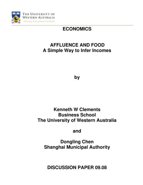
FIGURE 1RATIOS OF FOOD-BUDGET-SHARE CHANGESTO INCOME CHANGES( × 100 )250200Median = -12.6150100500-102.5-92.5 -82.5 -72.5 -62.5 -52.5 -42.5 -32.5 -22.5 -12.5 -2.5 7.5 17.5 27.5 37.5 47.5110100Median = -12.69080706050403020100-25 -23 -21 -19 -17 -15 -13 -11 -9 -7 -5 -3 -1 1 3 5 7FIGURE 223

SCATTER OF CHANGES IN FOOD BUDGET SHAREAGAINST INCOME CHANGES IN 42 COUNTRIESI. All pairs of countries∆ ×abw 100100 x (wa-wb)-30-25y = -0.1282x(0.0019)R 2 = 0.8479-20-15-10-5050 20 40 60 80 100 120 140 160 180 200a b100 100 × log x log(Qa/Qb)Q )10II. Five outlining pairs excluded∆ ×abw 100100 x (wa-wb)-30-25y = -0.1301x(0.0018)R 2 = 0.8617-20-15-10-5050 20 40 60 80 100 120 140 160 180 200a b100 × 100 logx (Qlog(Qa/Qb)Q )10Note: The 5 excluded pairs of countries in panel II are Malta with Turkey, Macedonia, Romania, Russia, and Bulgaria.24

FIGURE 3SCATTER OF FOOD BUDGET SHAREAGAINST INCOMEFood budget share( × 100)4, 000 8, 000 16, 000 32, 00025

TABLE 5THE FLORIDA MODEL: ESTIMATES AND SIMULATION RESULTSc⎡c 12c c c pp ⎤ic jwi = αi + βiq + ( αi + βiq ) ⎢log − ∑( αj+βjq ) log ⎥⎢⎣pij=1pj⎥⎦⎡p ⎤i+ φ ( α + β q ) ⎢log − ∑( α + β q ) log + ε⎢⎣⎥⎦c 12c*c p*c j ci i j j ⎥ ipij=1pjCommodity Data based Monte Carlo simulationIntercept αiSlope β iIntercept αiSlope β iPoint estimate ASE Point estimate ASE Mean RMSE RMASE Mean RMSE RMASE(1) (2) (3) (4) (5) (6) (7) (8) (9) (10) (11)1. Food 0.0789 0.0051 -0.1010 0.0059 0.0792 0.0051 0.0048 -0.1008 0.0061 0.00552. Alcohol & tobacco 0.0356 0.0042 -0.0073 0.0050 0.0356 0.0041 0.0040 -0.0073 0.0050 0.00463. Clothing 0.0453 0.0034 -0.0039 0.0036 0.0451 0.0035 0.0032 -0.0041 0.0038 0.00344. Housing 0.1511 0.0097 -0.0306 0.0123 0.1515 0.0104 0.0090 -0.0301 0.0132 0.01115. Durables 0.0553 0.0028 0.0084 0.0031 0.0553 0.0029 0.0026 0.0083 0.0032 0.00296. Health 0.1184 0.0067 0.0313 0.0094 0.1186 0.0070 0.0063 0.0315 0.0100 0.00867. Transport 0.1099 0.0049 0.0090 0.0055 0.1099 0.0051 0.0046 0.0091 0.0056 0.00508. Communication 0.0231 0.0019 -0.0049 0.0018 0.0230 0.0019 0.0018 -0.0049 0.0019 0.00169. Recreation 0.0978 0.0040 0.0301 0.0046 0.0978 0.0042 0.0038 0.0300 0.0048 0.004310. Education 0.0743 0.0062 -0.0019 0.0093 0.0744 0.0067 0.0055 -0.0017 0.0105 0.008011. Restaurants 0.0785 0.0080 0.0219 0.0094 0.0780 0.0082 0.0076 0.0213 0.0098 0.008712. Other 0.1320 0.0079 0.0488 0.0097 0.1317 0.0081 0.0075 0.0486 0.0100 0.0091Income flexibility Point estimate = -0.7728, ASE = 0.0533 Mean = -0.7754, RMSE = 0.0619, RMASE = 0.0446c cNotes: 1. q * = 1 + q2. The Monte Carlo simulation involves 1,000 trials.3. ASE = asymptotic standard error.4. RMSE is the root mean squared error over the 1,000 trials.1,000 (s)5. RMASE ( ) ( ) 2= 1 1000 ∑s = 1ASE where(s)ASE is the asymptotic SE of a given parameter at trial s.26

TABLE 6A CROSS-COUNTRY INCOME COMPARISONCountryclog ( Q*Q )cComponents of simulated log ( Q*Q )Observed Simulated Food share Food relative priceMean SD Mean SD Mean SD(1) (2) (3) (4) (5) (6) (7) (8)1. L'bourg 86.6 62.6 11.5 73.1 11.6 -10.6 0.72. USA 66.6 42.2 10.9 73.3 11.0 -31.1 2.03. UK 49.6 45.5 16.0 59.9 15.4 -14.4 0.74. S'land 42.3 43.3 18.0 46.8 17.8 -3.5 0.15. Austria 41.0 39.6 17.6 53.0 17.2 -13.4 0.66. Norway 38.5 40.6 19.2 41.4 19.2 -0.8 0.07. France 37.1 38.4 19.3 40.3 19.3 -1.9 0.18. Iceland 36.7 40.2 18.9 30.4 19.2 9.7 0.49. Denmark 35.5 37.5 18.2 47.4 17.9 -10.0 0.410. Sweden 34.3 36.6 17.6 46.6 17.3 -9.9 0.411. N'lands 34.0 33.5 18.3 47.4 17.8 -13.9 0.612. Canada 33.2 32.5 17.8 52.5 17.1 -20.0 0.913. Belgium 33.2 35.3 18.6 45.4 18.3 -10.1 0.414. Australia 31.6 33.1 18.9 44.5 18.5 -11.4 0.515. Italy 31.3 32.0 18.7 39.4 18.5 -7.4 0.316. Germany 28.6 28.8 18.9 46.9 18.3 -18.1 0.817. Cyprus 22.7 19.7 20.0 24.4 19.8 -4.7 0.218. Ireland 22.7 23.3 18.7 37.1 18.3 -13.7 0.619. Japan 21.6 25.5 20.3 2.5 20.8 23.1 0.920. Spain 21.0 20.2 20.1 32.1 19.8 -11.8 0.521. Finland 20.4 22.5 20.2 36.5 19.8 -14.0 0.622. NZ 12.3 14.0 20.2 16.9 20.1 -2.9 0.123. Israel 12.1 18.8 20.5 19.3 20.5 -0.5 0.024. Greece 7.3 3.7 20.9 10.6 20.8 -6.9 0.325. Malta 7.2 -1.3 20.9 0.6 20.9 -1.9 0.126. Portugal 3.4 -2.2 21.0 1.8 21.0 -4.0 0.227. Slovenia -5.9 -3.6 21.3 -11.7 21.4 8.1 0.328. Czech -12.5 -8.0 21.1 -13.0 21.2 4.9 0.229. Hungary -20.3 -19.4 20.4 -32.5 20.6 13.2 0.630. Korea -27.0 -20.6 20.1 -44.6 20.5 24 1.131. Slovakia -32.2 -28.1 20.4 -48.3 20.7 20.2 0.932. Croatia -35.5 -37.3 19.7 -60.0 20.1 22.7 1.133. Poland -37.7 -32.2 20.4 -30.2 20.4 -2.0 0.134. Lithuania -39.4 -40.2 19.9 -54.4 20.1 14.3 0.735. Estonia -41.8 -37.1 20.1 -55.0 20.3 17.9 0.836. Latvia -55.1 -49.4 18.9 -70.6 19.2 21.2 1.037. Mexico -63.3 -53.9 20.4 -41.2 20.2 -12.7 0.638. Bulgaria -82.6 -81.9 17.8 -110.2 18.3 28.3 1.539. Russia -83.9 -100.4 17.2 -114.4 17.4 14.1 0.840. Romania -86.9 -86.4 17.3 -109.9 17.7 23.5 1.241. Macedonia -91.0 -90.7 16.7 -109.2 16.9 18.5 1.042. Turkey -95.8 -91.3 17.0 -111.9 17.3 20.7 1.1Notes: 1. All entries are to be divided by 100.27

2. Q * = geometric mean of Q c3. SD=standard deviation.FIGURE 4ACTUAL AND PREDICTED INCOME(Logarithms × 100 )Actual100A = P500-150 -100 -50 0 50 100-50-100y = 0.355 + 1.027x, R0(1.067) (0.024)2Predicted= 0.978H : Intercept = 0, slope = 1F = 0.660-15028

FIGURE 5OBSERVED AND SIMULATED CROSS-COUNTRY INCOME COMPARISONSI. ObservedII. Simulated29

FIGURE 6TWO MEASURES OF INCOME DIFFERENCES100Log ratio of realincome of countryto geometric mean× 100500-50Unadjusted for pricesAdjusted for prices-100-150Poorer-30Log ratio of realincome of countryto geometric mean× 100-60CountryAdjusted for prices-90-120Unadjusted for pricesPoorer-150Country30

FIGURE 7MATRIX OF HISTOGRAMS OF SIMULATED INCOME DIFFERENCES FOR SIX COUNTRY GROUPS( Logarithmic ratios × 100)← POORER RICHER →Group 6 Group 5 Group 4 Group 3 Group 2300300300300300Group 12001000-17.5 17.5 52.5 87.5 122.52001000-17.5 17.5 52.5 87.5 122.52001000-17.5 17.5 52.5 87.5 122.52001000-17.5 17.5 52.5 87.5 122.52001000-17.5 17.5 52.5 87.5 122.5300300300300← POORER RICHER →Group 4Group 3Group 22001000-17.5 17.5 52.5 87.5 122.53002001000-17.5 17.5 52.5 87.5 122.53002001000-17.5 17.5 52.5 87.5 122.52001000-17.5 17.5 52.5 87.5 122.53002001000-17.5 17.5 52.5 87.5 122.53002001000-17.5 17.5 52.5 87.5 122.52001000-17.5 17.5 52.5 87.5 122.53002001000-17.5 17.5 52.5 87.5 122.52001000-17.5 17.5 52.5 87.5 122.5300Group 52001000-17.5 17.5 52.5 87.5 122.531

TABLE 7SIMULATED INCOME DIFFERENCES FORSIX COUTNRY GROUPS← POORER RICHER →GroupGroup 6 Group 5 Group 4 Group 3 Group 2Mean SD( )P Q G > Q 6Mean SD( )P Q G > Q 5Mean SD( )P Q G > Q 4Mean SD( )P Q G > Q 3Mean SD( )P Q G > Q 2RICHER →← POORER1 123.7 7.7 1.000 75.3 9.2 1.000 41.5 10.1 1.000 20.0 9.9 0.980 9.1 9.3 0.8342 114.6 7.9 1.000 66.2 9.6 1.000 32.5 10.3 1.000 10.9 10.1 0.8673 103.7 8.4 1.000 55.2 10.3 1.000 21.5 10.6 0.9794 82.2 9.7 1.000 33.7 10.8 0.9985 48.4 10.2 1.000Notes: 1. SD = standard deviation.2. In all cases, the underlying variable is the logarithmic ratio of real incomes × 100 .3. ( G HP Q Q )> is the probability that income of country group G exceeds that of H, for G < H, G = 1,…,5, and H = 2,…,6.32

FIGURE 8PROBABILITY OF INCOME DIFFERENCES(c+x>c)P Q Q10.80.60.4L'bourg (1)N'lands (11)0.2Turkey (42)Croatia (32)NZ (22)Canada (12)USA (2)Finland (21)Slovakia (31)Macedonia (41)33

TABLE 8PROBABILITY OF INCOME DIFFERENCES BYDISTANCE BETWEEN COUNTRIESDistance as measured Probability that country c is richer than c+xby band width(Number of countries) Marginal Cumulativexc c+xc c+yx P( Q > Q ) ∑ P ( Q > Q )y=0(1) (2) (3)0 0.000 0.0001 0.553 0.2732 0.594 0.3773 0.633 0.4394 0.682 0.4855 0.719 0.5226 0.747 0.5517 0.777 0.5778 0.799 0.5999 0.823 0.61910 0.836 0.63611 0.856 0.65112 0.872 0.66613 0.887 0.67914 0.904 0.69115 0.918 0.70216 0.925 0.71217 0.934 0.72118 0.945 0.73019 0.956 0.73820 0.967 0.74521 0.972 0.75222 0.980 0.75823 0.987 0.76424 0.989 0.77025 0.992 0.77526 0.996 0.77927 0.997 0.78328 0.999 0.78729 0.999 0.7930 0.999 0.79331 1.000 0.79632 1.000 0.79833 1.000 0.80034 1.000 0.80235 1.000 0.80436 1.000 0.80537 1.000 0.80638 1.000 0.80739 1.000 0.80840 1.000 0.80841 1.000 0.808Notes:1. Countries are indexed by c = 1,…,42 and ranked in terms of decreasing per capitaincome. Column 2 gives the relative frequency that country c is richer than country c+x(x ≥ 0, the "band width") , for c = 1, ..., 42. Alternatively, in the 1,000 realisations ofthe 42 × 42 matrix⎡⎣⎤⎦Q (s) a(s) b(s)= Q - Q , s = 1, ...,1, 000 , the entry in column 2corresponding to band width x, is the average of the relative frequencies on the subdiagonal x steps away from the main diagonal once removed.2. Column 3 gives the relative frequencies of positive values contained in the bands of(s)Q , s = 1, ...,1, 000 , x steps away from the main diagonal once removed.34

TABLE 9COMPARISON OF ROMANIA AND FRANCEConcept(1)Ratio of food shares:wRwFObserved(2)2.72Priceadjusted(3)RR⎧⎪⎛ w ⎞ ⎛ w ⎞⎫⎪exp ⎨log⎜ logF ⎟ − ∆ ⎜ F ⎟⎬⎪⎩⎝ w ⎠ ⎝ w ⎠⎪⎭2.35Estimated income difference:R1 ⎛ w ⎞logRF ⎜ F ⎟η −1 ⎝ w ⎠-1.67RR1 ⎧⎪⎛ w ⎞ ⎛ w ⎞⎫⎪log logRF ⎨ ⎜ F ⎟ − ∆ ⎜ F ⎟⎬η −1⎪⎩⎝ w ⎠ ⎝ w ⎠⎪⎭-1.42Percentage difference -81% -76%35

TABLE A1BUDGET SHARES OF 12 GOODS IN 42 COUNTRIES(Percentages)FoodAlcohol &tobaccoClothingHousingDurablesCountry(1) (2) (3) (4) (5) (6) (7) (8) (9) (10) (11) (12) (13)1. L'bourg 7.7 9.4 3.8 17.3 6.5 7.6 14.7 1.4 8.1 7.2 6.0 10.12. USA 6.4 2.0 4.3 16.4 4.4 17.8 10.5 1.7 8.5 8.5 5.5 13.83. UK 7.6 3.2 4.9 14.7 4.9 9.2 11.7 1.8 10.7 5.7 9.5 16.14. S'land 9.6 3.2 3.7 20.7 4.1 12.8 7.0 2.0 8.7 7.7 6.8 13.85. Austria 8.8 2.4 5.5 16.1 6.6 9.7 10.6 2.1 9.6 8.0 9.7 10.96. Norway 10.6 3.4 4.3 15.4 4.7 13.6 10.8 2.1 11.3 8.2 4.7 10.97. France 11.4 2.7 3.7 19.5 4.8 12.9 11.7 1.8 8.0 6.8 6.0 10.88. Iceland 13.9 3.6 4.2 14.9 5.3 14.1 8.7 0.9 10.0 8.7 6.4 9.19. Denmark 8.8 3.1 3.6 20.2 4.1 10.1 8.5 1.5 9.1 9.7 3.8 17.410. Sweden 8.7 2.9 3.9 19.8 3.5 11.2 8.9 2.3 10.1 10.0 3.5 15.111. N'lands 8.7 2.4 4.6 16.7 5.6 10.4 9.4 3.1 9.6 7.1 4.5 17.812. Canada 8.0 3.3 4.2 19.3 5.4 12.0 12.1 1.8 9.6 7.9 6.1 10.313. Belgium 10.4 2.9 4.3 18.2 4.4 12.3 11.0 1.8 8.0 9.4 4.2 13.014. Australia 9.2 3.7 3.4 17.9 5.2 12.2 10.1 2.4 10.6 6.8 6.8 11.615. Italy 12.2 2.0 7.7 16.5 7.4 10.9 9.9 2.5 6.8 7.0 8.1 8.816. Germany 9.8 3.2 4.9 20.0 5.4 12.5 11.7 2.3 8.2 5.8 3.8 12.317. Cyprus 13.6 4.3 6.4 11.8 5.9 5.4 13.3 2.2 7.5 6.2 11.7 11.718. Ireland 6.3 5.2 4.9 17.3 5.6 9.7 8.3 2.1 6.2 9.9 13.8 10.819. Japan 12.3 2.5 3.9 22.0 3.7 12.3 8.9 2.3 7.9 6.4 6.2 11.620. Spain 13.5 2.7 5.3 12.2 4.9 9.7 10.3 2.3 7.7 6.7 16.5 8.121. Finland 9.6 4.4 3.5 19.2 3.7 11.1 9.2 2.5 9.7 8.3 4.9 13.922. NZ 11.4 4.1 4.0 18.5 5.3 9.4 11.6 2.5 11.6 6.7 6.6 8.323. Israel 14.6 2.1 2.7 20.9 5.8 10.2 7.8 3.2 6.9 12.4 3.0 10.324. Greece 14.5 4.3 9.5 14.4 5.9 8.1 7.3 2.6 5.5 6.3 15.9 5.625. Malta 16.0 3.1 5.1 7.9 7.7 7.7 12.2 4.1 8.7 7.5 12.0 7.826. Portugal 15.1 3.3 5.8 8.8 5.9 11.3 13.7 3.0 6.7 8.9 8.0 9.727. Slovenia 13.9 3.8 5.1 16.3 5.0 10.9 12.0 2.2 8.8 8.2 5.3 8.428. Czech 14.1 7.1 4.3 18.5 4.4 10.6 8.2 2.4 10.7 7.1 5.4 7.129. Hungary 15.1 6.8 3.5 14.4 5.4 11.1 12.0 4.1 7.8 7.9 3.9 7.930. Korea 13.4 2.1 4.1 14.4 3.9 4.1 10.3 5.2 7.5 9.4 6.7 18.931. Slovakia 19.2 4.8 3.7 20.0 4.5 9.1 8.0 3.3 9.0 5.8 6.5 6.132. Croatia 22.3 5.4 5.7 16.5 4.5 6.7 11.5 2.7 4.8 6.5 6.3 7.433. Poland 17.7 5.7 4.0 21.5 3.9 8.7 9.2 2.8 6.7 7.6 2.6 9.634. Lithuania 23.8 5.9 5.1 14.4 4.3 9.2 11.6 2.8 6.4 7.7 2.8 6.135. Estonia 18.4 7.9 5.2 19.9 4.1 6.7 9.5 2.5 7.3 8.2 4.6 5.836. Latvia 21.3 6.6 6.4 18.5 2.6 8.6 7.8 3.1 8.0 8.7 4.0 4.237. Mexico 21.7 2.4 3.1 11.9 7.5 7.0 15.3 1.5 3.0 8.9 7.0 10.838. Bulgaria 22.9 2.8 3.2 20.5 2.9 7.0 13.8 5.3 4.8 5.6 7.6 3.539. Russia 27.3 7.4 10.9 6.8 4.6 8.2 9.3 3.2 4.9 7.0 2.4 7.940. Romania 31.0 4.8 3.2 20.7 3.7 6.9 10.2 2.7 4.9 4.0 4.3 3.641. Macedonia 29.8 3.6 5.5 16.4 3.9 7.9 10.2 5.2 2.7 5.2 3.4 6.242. Turkey 24.6 3.8 5.8 25.5 6.8 3.6 8.2 4.2 2.4 5.6 4.2 5.3HealthTransportCommRecreationEducationRestaurantsOther36

TABLE A2PPP PRICES OF 12 COMMODITIES IN 42 COUNTRIES(Domestic-currency cost of a US dollar’s worth of each good)FoodAlcohol &tobaccoClothingHousingDurablesCountry(1) (2) (3) (4) (5) (6) (7) (8) (9) (10) (11) (12) (13)1. L'bourg 1.07 0.82 1.29 1.12 1.10 0.84 1.08 0.81 1.16 1.32 1.04 1.002. USA 0.95 1.02 0.95 1.17 1.05 1.59 0.87 0.99 0.95 1.88 0.97 1.073. UK 0.67 1.22 0.58 0.48 0.77 0.48 0.93 0.78 0.75 0.59 0.80 0.664. S'land 2.24 1.67 1.86 2.34 1.81 1.67 2.11 1.74 2.25 1.84 2.22 1.925. Austria 1.01 0.99 1.17 0.83 1.09 0.77 1.33 1.06 1.16 0.86 1.06 1.096. Norway 12.04 20.12 10.34 7.52 10.15 8.24 15.53 8.86 12.55 8.29 13.44 11.397. France 1.09 1.05 1.00 1.07 0.96 0.67 1.17 1.20 1.09 0.68 0.98 0.968. Iceland 134.00 177.90 113.70 79.40 115.90 77.50 128.50 69.10 142.50 74.70 152.90 106.909. Denmark 9.70 10.71 9.09 8.82 8.82 7.07 13.37 7.37 10.45 7.80 10.92 9.8710. Sweden 10.56 13.51 10.98 9.60 11.68 7.59 13.57 7.25 11.93 7.98 11.56 10.8611. N'lands 0.98 0.98 1.17 1.02 1.05 0.68 1.34 0.94 1.02 0.76 1.05 0.9612. Canada 1.33 2.09 1.51 1.33 1.62 1.18 1.46 1.04 1.62 1.44 1.55 1.3613. Belgium 1.00 0.95 1.20 0.92 0.99 0.75 1.16 1.15 1.07 0.81 1.02 1.0014. Australia 1.54 2.28 1.67 1.54 1.56 1.05 1.69 1.44 1.73 1.22 1.55 1.5415. Italy 1.00 0.89 1.09 0.77 1.03 0.77 1.14 1.23 1.11 0.71 1.05 0.9116. Germany 1.01 0.92 1.16 1.06 1.02 0.85 1.32 1.00 1.12 1.05 0.93 1.0617. Cyprus 0.56 0.66 0.57 0.35 0.55 0.40 0.65 0.37 0.60 0.39 0.65 0.4518. Ireland 1.14 1.74 0.90 1.27 1.08 0.79 1.41 1.08 1.21 0.85 1.34 1.0719. Japan 0.24 0.13 0.17 0.21 0.16 0.11 0.16 0.15 0.14 0.15 0.19 0.1620. Spain 0.83 0.71 1.17 0.68 1.01 0.57 1.08 1.04 0.98 0.55 0.89 0.7321. Finland 1.14 1.66 1.16 1.09 1.13 0.82 1.49 1.09 1.37 0.88 1.31 1.1722. NZ 1.86 2.73 2.05 1.67 2.12 1.00 1.98 1.55 1.83 1.02 1.70 1.6223. Israel 4.69 5.05 4.11 5.12 3.66 2.73 5.53 3.71 5.05 2.67 5.02 3.9224. Greece 0.84 0.87 1.21 0.63 0.88 0.43 0.92 1.06 0.95 0.45 0.90 0.7325. Malta 0.33 0.47 0.35 0.15 0.37 0.18 0.39 0.58 0.37 0.18 0.32 0.2626. Portugal 0.85 0.81 0.88 0.36 0.79 0.52 1.18 1.20 0.93 0.70 0.81 0.7827. Slovenia 195.60 151.70 209.50 133.30 159.10 105.60 226.10 156.60 206.80 113.30 155.20 151.7028. Czech 17.64 18.91 26.20 10.71 21.61 8.50 25.86 29.70 18.59 7.20 15.59 13.4529. Hungary 0.16 0.15 0.19 0.08 0.16 0.06 0.24 0.24 0.16 0.06 0.14 0.1030. Korea 1.30 0.94 0.96 1.12 0.90 0.56 0.96 0.76 0.97 0.68 0.89 0.8131. Slovakia 22.70 23.58 29.72 10.06 26.69 9.14 31.00 45.46 20.71 6.88 14.57 14.7732. Croatia 5.80 5.50 5.77 1.74 4.99 2.78 7.04 6.16 5.20 2.54 5.03 3.9133. Poland 2.18 3.05 3.28 1.28 2.69 1.13 3.41 5.36 2.81 0.92 2.72 1.9434. Lithuania 2.08 2.24 2.82 0.93 2.31 0.72 2.80 5.39 2.11 0.53 2.25 1.3135. Estonia 11.12 10.42 14.10 6.55 10.99 4.11 12.64 13.10 10.74 2.84 11.33 7.0036. Latvia 0.38 0.38 0.45 0.19 0.41 0.13 0.47 0.76 0.36 0.10 0.40 0.2537. Mexico 7.49 7.92 9.23 10.33 6.97 4.15 8.19 13.44 8.65 4.19 7.80 7.4638. Bulgaria 1.05 0.79 1.10 0.44 0.94 0.36 1.30 1.53 0.96 0.17 0.69 0.5839. Russia 13.10 10.80 20.00 3.40 18.40 2.90 15.10 23.00 13.50 3.00 15.70 10.8040. Romania 16.17 12.94 13.02 7.74 15.60 5.00 19.18 29.96 14.58 2.68 12.72 8.1941. Macedonia 30.00 21.30 30.00 13.60 30.60 9.40 40.50 33.30 28.70 9.30 23.20 21.2042. Turkey 903.94 789.09 1029.75 385.86 856.43 364.25 1086.31 2092.93 918.79 243.11 642.38 634.68Note: Nominal prices are in thousands for Japan, Hungary, Korea, Romania, and Turkey.HealthTransportCommRecreationEducationRestaurantsOther37

TABLE A3VOLUME OF CONSUMPTION PER CAPITA OF 12 GOODS IN 42 COUNTRIES(US dollars)FoodAlcohol &tobaccoClothingHousingDurablesHealthCountry(1) (2) (3) (4) (5) (6) (7) (8) (9) (10) (11) (12) (13) (14)1. L'bourg 2,247 3,655 937 4,870 1,883 2,863 4,323 547 2,211 1,738 1,812 3,173 30,2582. USA 1,884 560 1,273 3,900 1,180 3,121 3,384 491 2,519 1,259 1,593 3,606 24,7683. UK 1,550 361 1,139 4,148 873 2,607 1,716 319 1,945 1,313 1,611 3,317 20,8994. S'land 1,670 752 769 3,459 886 3,000 1,298 444 1,511 1,624 1,196 2,815 19,4245. Austria 1,664 464 896 3,694 1,152 2,387 1,524 373 1,584 1,773 1,748 1,904 19,1616. Norway 1,682 320 798 3,923 893 3,163 1,331 447 1,724 1,901 670 1,839 18,6917. France 1,839 442 644 3,196 869 3,350 1,741 266 1,289 1,764 1,073 1,966 18,4398. Iceland 1,955 385 705 3,542 868 3,444 1,278 236 1,330 2,205 795 1,615 18,3589. Denmark 1,522 489 656 3,837 778 2,387 1,060 335 1,461 2,076 588 2,954 18,14510. Sweden 1,474 379 640 3,702 534 2,655 1,182 558 1,514 2,253 546 2,497 17,93411. N'lands 1,527 423 681 2,799 920 2,615 1,205 576 1,612 1,599 732 3,181 17,87112. Canada 1,497 389 694 3,595 828 2,538 2,050 442 1,478 1,357 979 1,888 17,73613. Belgium 1,766 518 605 3,335 759 2,771 1,602 258 1,261 1,951 701 2,209 17,73514. Australia 1,540 424 527 3,002 871 3,013 1,545 430 1,583 1,431 1,132 1,945 17,44315. Italy 1,963 360 1,131 3,454 1,163 2,275 1,391 329 984 1,577 1,236 1,541 17,40316. Germany 1,726 620 753 3,330 941 2,588 1,561 403 1,284 969 725 2,042 16,94117. Cyprus 1,932 520 900 2,739 869 1,079 1,644 472 1,000 1,263 1,442 2,108 15,96918. Ireland 976 527 961 2,407 930 2,193 1,043 346 909 2,054 1,836 1,783 15,96519. Japan 1,339 489 595 2,786 607 2,863 1,438 394 1,451 1,109 837 1,881 15,78820. Spain 2,020 469 566 2,232 612 2,135 1,190 273 983 1,507 2,319 1,396 15,70121. Finland 1,476 467 522 3,076 568 2,375 1,082 403 1,236 1,651 651 2,088 15,59622. NZ 1,428 347 449 2,571 577 2,201 1,358 379 1,473 1,521 895 1,189 14,39023. Israel 1,776 233 371 2,336 911 2,140 808 493 780 2,660 342 1,509 14,35824. Greece 1,762 507 806 2,322 683 1,940 812 252 591 1,426 1,800 791 13,69125. Malta 1,821 253 566 2,063 788 1,657 1,205 270 889 1,598 1,417 1,144 13,66926. Portugal 1,702 382 628 2,303 717 2,068 1,111 236 681 1,211 941 1,177 13,15627. Slovenia 1,308 467 451 2,254 585 1,902 977 264 788 1,337 634 1,027 11,99328. Czech 1,217 577 252 2,637 308 1,897 486 126 878 1,515 526 811 11,22929. Hungary 1,090 514 210 2,088 386 1,960 572 197 562 1,619 328 852 10,38130. Korea 903 193 371 1,118 382 651 934 597 671 1,199 654 2,044 9,71731. Slovakia 1,146 275 170 2,697 231 1,345 351 100 588 1,147 604 564 9,21832. Croatia 1,256 319 324 3,106 295 783 532 141 302 837 408 616 8,91833. Poland 1,243 287 185 2,573 224 1,174 414 79 368 1,281 147 756 8,72934. Lithuania 1,328 306 209 1,796 215 1,476 481 59 350 1,681 142 537 8,58135. Estonia 1,021 467 227 1,882 233 1,007 462 117 422 1,773 249 514 8,37436. Latvia 978 304 249 1,738 114 1,204 293 73 394 1,506 179 297 7,33037. Mexico 1,377 142 157 546 510 801 884 52 165 1,009 424 688 6,75638. Bulgaria 729 118 99 1,539 104 642 353 116 169 1,127 370 203 5,56739. Russia 899 297 237 859 108 1,214 268 59 157 1,021 65 315 5,49940. Romania 1,015 196 132 1,420 125 736 282 47 177 793 181 231 5,33641. Macedonia 1,014 175 189 1,229 132 852 257 159 95 573 149 300 5,12342. Turkey 773 136 159 1,882 227 282 213 57 76 653 185 237 4,882Note: Totals may not check due to rounding.TransportCommRecreationEducationRestaurantsOtherTotal38

TABLE A4RELATIVE PPP PRICES FOR 12 COMMODITIES IN 42 COUNTRIESLogarithmic ratios×100( )FoodAlcohol &tobaccoClothingHousingDurablesCountry(1) (2) (3) (4) (5) (6) (7) (8) (9) (10) (11) (12) (13)1. L'bourg 2.1 -25.5 20.5 6.4 4.1 -22.5 2.2 -26.0 9.9 22.4 -1.0 -5.22. USA -19.7 -12.7 -20.2 1.1 -9.6 31.9 -29.2 -15.8 -20.3 48.4 -18.3 -7.83. UK -0.9 59.3 -14.3 -32.9 14.1 -33.0 32.9 14.4 11.1 -13.3 17.9 -1.54. S'land 10.1 -19.6 -8.8 14.2 -11.5 -19.3 4.0 -15.3 10.2 -9.5 8.9 -5.45. Austria 0.3 -2.0 15.2 -19.5 8.1 -26.6 27.5 4.6 13.8 -15.8 4.7 7.66. Norway 12.7 64.1 -2.5 -34.3 -4.4 -25.2 38.2 -17.9 16.9 -24.6 23.8 7.27. France 11.7 8.4 3.0 9.6 -0.6 -36.5 19.3 21.5 12.2 -35.6 1.3 -0.98. Iceland 22.6 50.9 6.2 -29.6 8.0 -32.2 18.3 -43.3 28.7 -35.8 35.9 0.09. Denmark 3.8 13.7 -2.7 -5.7 -5.7 -27.8 35.8 -23.7 11.2 -18.0 15.6 5.510. Sweden 3.9 28.5 7.7 -5.7 13.9 -29.2 28.9 -33.7 16.1 -24.2 12.9 6.711. N'lands 0.0 0.4 18.1 4.8 7.1 -36.1 32.0 -4.0 4.8 -24.7 7.2 -1.312. Canada -6.1 39.2 6.8 -5.7 13.5 -18.2 3.6 -30.9 13.7 2.1 9.1 -4.113. Belgium 3.7 -1.1 21.9 -4.1 2.6 -24.7 19.0 18.1 10.5 -17.0 5.4 3.714. Australia 2.5 41.4 10.4 2.3 3.4 -36.2 11.6 -4.2 14.2 -20.7 3.1 2.615. Italy 6.4 -4.4 15.3 -19.8 9.5 -19.2 20.4 27.8 17.4 -26.9 12.2 -2.616. Germany -4.1 -12.6 9.8 0.9 -2.6 -20.5 22.9 -4.9 7.1 0.1 -11.6 1.217. Cyprus 9.1 24.5 9.5 -40.0 5.8 -25.5 23.3 -33.1 15.7 -27.8 23.3 -14.718. Ireland 0.4 42.8 -23.1 11.4 -5.5 -37.0 21.8 -5.1 6.0 -28.7 16.2 -6.119. Japan 34.5 -25.0 1.8 19.4 -7.2 -41.6 -5.2 -10.4 -17.2 -12.2 13.6 -5.120. Spain 2.3 -14.3 36.5 -17.7 21.3 -35.9 27.9 24.2 18.6 -38.8 8.4 -11.321. Finland 0.2 37.4 1.4 -4.5 -1.4 -32.9 26.4 -5.0 18.1 -25.8 13.8 2.022. NZ 10.8 49.2 20.7 0.3 24.2 -51.5 17.0 -7.4 9.4 -49.2 2.1 -2.923. Israel 13.0 20.4 -0.4 21.7 -11.8 -41.2 29.4 -10.4 20.3 -43.3 19.8 -5.124. Greece 7.2 11.4 43.4 -21.1 11.9 -60.2 16.9 30.8 19.9 -54.5 14.3 -7.325. Malta 11.7 45.8 14.5 -71.3 21.5 -51.9 26.0 66.7 22.5 -51.0 8.2 -14.126. Portugal 9.8 5.8 13.3 -74.5 2.5 -38.6 42.9 44.7 19.6 -9.0 5.0 2.027. Slovenia 20.7 -4.7 27.6 -17.6 0.0 -40.9 35.3 -1.5 26.3 -33.8 -2.4 -4.728. Czech 17.9 24.8 57.4 -32.0 38.2 -55.1 56.1 70.0 23.1 -71.8 5.5 -9.329. Hungary 25.1 19.5 44.5 -45.0 25.8 -64.8 66.6 66.0 25.0 -79.9 10.3 -15.730. Korea 34.4 2.5 4.5 19.8 -1.9 -50.4 4.5 -18.4 5.9 -29.8 -3.5 -12.931. Slovakia 31.0 34.8 57.9 -50.3 47.2 -59.9 62.2 100.4 21.9 -88.4 -13.3 -12.032. Croatia 33.0 27.9 32.6 -87.6 18.1 -40.6 52.5 39.0 22.2 -49.4 18.8 -6.433. Poland 11.7 45.1 52.6 -41.8 32.6 -53.9 56.4 101.7 37.0 -75.2 33.7 0.034. Lithuania 25.8 33.2 56.2 -54.8 36.4 -80.5 55.5 121.2 27.5 -110.3 33.9 -20.335. Estonia 29.0 22.4 52.7 -24.0 27.6 -70.7 41.8 45.0 25.4 -107.5 30.8 -17.336. Latvia 31.6 31.4 48.4 -39.8 37.7 -79.8 52.1 99.1 25.1 -101.1 34.7 -11.137. Mexico 2.4 8.0 23.2 34.5 -4.8 -56.6 11.3 60.8 16.7 -55.7 6.4 1.938. Bulgaria 37.1 8.4 41.9 -48.7 25.8 -69.1 58.7 74.5 28.1 -147.3 -4.9 -21.939. Russia 25.2 5.7 66.9 -109.7 58.7 -124.8 38.9 81.2 28.2 -123.2 43.1 5.740. Romania 33.1 10.8 11.4 -40.5 29.5 -84.3 50.2 94.8 22.7 -146.7 9.1 -34.941. Macedonia 28.9 -5.4 29.0 -50.2 30.8 -86.9 58.7 39.1 24.2 -88.8 3.1 -5.642. Turkey 30.7 17.1 43.7 -54.4 25.3 -60.2 49.1 114.7 32.3 -100.6 -3.5 -4.7HealthTransportCommRecreationEducationRestaurantsOther39

TABLE A5CONSUMPTION AND GDP PER CAPITA IN 42 COUNTRIESCountry Consumption per capita GDP per capita(US dollars) Using PPP Using market exchange ratesIndexIndexUS dollars (L’bourg = 100) US dollars (L’bourg = 100)(1) (2) (3) (4) (5) (6)1. L'bourg 30,258 47,271 100.0 48,104 100.02. USA 24,768 32,798 69.4 36,202 75.33. UK 20,899 26,188 55.4 26,393 54.94. S'land 19,424 29,449 62.3 37,624 78.25. Austria 19,161 27,270 57.7 25,818 53.76. Norway 18,691 33,232 70.3 42,035 87.47. France 18,439 25,096 53.1 23,455 48.88. Iceland 18,358 26,594 56.3 29,550 61.49. Denmark 18,145 27,217 57.6 32,059 66.610. Sweden 17,934 25,504 54.0 27,084 56.311. N'lands 17,871 27,123 57.4 25,935 53.912. Canada 17,736 26,807 56.7 23,176 48.213. Belgium 17,735 25,938 54.9 23,780 49.414. Australia 17,443 25,276 53.5 20,255 42.115. Italy 17,403 24,219 51.2 20,745 43.116. Germany 16,941 24,148 51.1 24,034 50.017. Cyprus 15,969 18,556 39.3 14,677 30.518. Ireland 15,965 29,789 63.0 30,993 64.419. Japan 15,788 24,648 52.1 31,170 64.820. Spain 15,701 21,014 44.5 16,208 33.721. Finland 15,596 25,192 53.3 25,287 52.622. NZ 14,390 19,875 42.0 14,874 30.923. Israel 14,358 20,490 43.3 16,529 34.424. Greece 13,691 17,275 36.5 12,157 25.325. Malta 13,669 16,500 34.9 10,270 21.326. Portugal 13,156 17,069 36.1 11,668 24.327. Slovenia 11,993 16,729 35.4 11,095 23.128. Czech 11,229 15,025 31.8 7,232 15.029. Hungary 10,381 13,013 27.5 6,383 13.330. Korea 9,717 16,709 35.3 11,481 23.931. Slovakia 9,218 11,418 24.2 4,503 9.432. Croatia 8,918 9,583 20.3 5,046 10.533. Poland 8,729 10,141 21.5 4,985 10.434. Lithuania 8,581 9,421 19.9 4,050 8.435. Estonia 8,374 10,195 21.6 5,164 10.736. Latvia 7,330 8,655 18.3 3,939 8.237. Mexico 6,756 8,489 18.0 6,390 13.338. Bulgaria 5,567 6,400 13.5 1,984 4.139. Russia 5,499 7,327 15.5 2,392 5.040. Romania 5,336 6,357 13.4 2,089 4.341. Macedonia 5,123 5,464 11.6 1,877 3.942. Turkey 4,882 5,903 12.5 2,605 5.440