Using Rotations to Build Aerospace Coordinate Systems - Defence ...

Using Rotations to Build Aerospace CoordinateSystemsDon KoksElectronic Warfare and Radar DivisionSystems Sciences LaboratoryDSTO–TN–0640ABSTRACTPresented here are the main techniques necessary to understand rotations inthree dimensions, for use with global visualisation and aerospace simulations.Relevant techniques can be extremely difficult to find in textbooks, so someuseful examples are collected here to highlight these techniques.The three standard aerospace coordinate systems are described and builtusing rotations. The mathematics of rotations is described, using both matricesand quaternions. The necessary calculations are given for analysing standardscenarios that involve the Global Positioning Satellite system for finding lineof-sightdirections on Earth, as well as for visualising the world from a cockpit,and for converting to and from the standard software protocol for distributedinteractive simulation environments.Appendices then discuss combining rotations, conversions with a particulartype of Euler angle convention, the dangers of confusing Euler angles withincremental rotations for software writers, and finally there is a short dicussionof interpolation of rotations in computing.APPROVED FOR PUBLIC RELEASE

DSTO–TN–0640Using Rotations to Build Aerospace Coordinate SystemsEXECUTIVE SUMMARYThis paper presents the main techniques necessary to understand three-dimensional rotations.The subject is not new, but can be very difficult to sort out and to explore intextbooks. Mathematics and physics texts that discuss the subject generally do so only inpassing, and probably never cover any standard software protocols. The main literatureon the subject seems to be that generated by the graphics computing community, sinceprogrammers need to use rotations when writing three-dimensional visualisation code.Nevertheless, code ease-of-use and ability to be passed on means that although there aremany internet sites that talk about rotations, their information content is often biasedtowards whatever system or code their authors have become familiar with.We begin by describing the three standard coordinate systems that are used for simulationof aerospace scenarios and the Global Positioning Satellite system, and how theirdefining axes can be built from rotations alone. We then describe the mathematics ofrotations using both matrices and quaternions, defining Euler angles, and concentratingon the important matrix (or equivalently, quaternion) that allows any rotation about anyaxis to be made.As examples of the techniques, we give the necessary calculations for dealing withstandard scenarios involving the Global Positioning Satellite system, for finding line-ofsightdirections on Earth, for visualising the world from a cockpit, and for converting to andfrom the standard software protocol for distributed interactive simulation environments.Appendices then discuss combining rotations, conversions with a particular type ofEuler angle convention, the dangers of confusing Euler angles with incremental rotationsfor software writers, and finally there is a short dicussion of interpolation of rotations incomputing.iii

DSTO–TN–0640iv

DSTO–TN–0640AuthorDon KoksElectronic Warfare and Radar DivisionDon Koks completed a doctorate in mathematical physics atAdelaide University in 1996, with a dissertation describing theuse of quantum statistical methods to analyse decoherence, entropyand thermal radiance in both the early universe and blackhole theory. He holds a Bachelor of Science from the Universityof Auckland in pure and applied mathematics, and a Masterof Science in physics from the same university with a thesisin applied accelerator physics (proton-induced X-ray and γ-rayemission for trace element analysis). He has worked on the acceleratormass spectrometry programme at the Australian NationalUniversity in Canberra, as well as in commercial internetdevelopment. Currently he is a Research Scientist with theMaritime Systems group in the Electronic Warfare and RadarDivision at DSTO, specialising in data fusion, geolocation, andthree-dimensional rotations.v

DSTO–TN–0640vi

DSTO–TN–0640ContentsGlossary, Conventions, and Constantsix1 Introduction 12 Important Coordinate Systems 12.1 ECEF: the Earth-Centred, Earth-Fixed Frame . . . . . . . . . . . . . . . 22.2 The Local Geographic Frame . . . . . . . . . . . . . . . . . . . . . . . . . 42.3 An Aircraft’s Own Frame . . . . . . . . . . . . . . . . . . . . . . . . . . . 53 The Basic Tool: Vector Rotations 53.1 Matrix Representation of an Orientation . . . . . . . . . . . . . . . . . . . 53.2 Euler Angles . . . . . . . . . . . . . . . . . . . . . . . . . . . . . . . . . . 63.3 The Workhorse: Rotating in Three Dimensions . . . . . . . . . . . . . . . 73.4 Rotating using Quaternions . . . . . . . . . . . . . . . . . . . . . . . . . . 94 Rotating Axes to Change Coordinates 114.1 Constructing NED Axes for the Local Geographic Frame . . . . . . . . . 124.2 The World as Seen by a Pilot . . . . . . . . . . . . . . . . . . . . . . . . . 154.3 ECEF Coordinates and Heading-Pitch-Roll Conversion . . . . . . . . . . 175 Concluding Remarks 20References 20AppendicesA Combining Two Rotations 21B xyz Eulers to Angle–Axis and Vice Versa 23C Confusing Euler Angle Orientation with Incremental Rotation 25D Quaternions Used in Computing: slerp 29vii

DSTO–TN–0640viii

DSTO–TN–0640Glossary, Conventions, and Constantsα Latitude of a point in the ECEF frame.ω Longitude of a point in the ECEF frame.Aircraft’s own axes x, y, z.Aircraft’s own axes as vectors in ECEF x, y, z.Earth’s elliptical cross-section This is defined by the following numbers:Semi-major: a = 6,378,137 m; semi-minor: b = 6,356,752.3142 m.ECEF Earth-Centred, Earth-Fixed Frame. A rotating frame fixed to Earth; the globalframe of this report within which all computations are done.ECEF Cartesian Axes X, Y, Z.Three Euler rotations act on a set of orthonormal vectors x 0 , y 0 , z 0 to give, in order,x 1 , y 1 , z 1 , then x 2 , y 2 , z 2 , and finally x 3 , y 3 , z 3 .GPS Global Positioning Satellite System.Local Geographic Frame A frame based at our current position, usually on or nearEarth’s surface. Two common choices for its axes are:NED North-East-Down set of axes.ENU East-North-Up set of axes.n A unit vector pointing along an axis of rotation. A column when used with matrices,and a row when used with quaternions. This might seem potentially confusing, butthere’s no ambiguity in practice; on the contrary, to continually write n and n t (thetranspose) just to emphasise a column or row would be tedious.North, East, Down axes N, E, D.North, East, Down axes as vectors in ECEF N, E, D.Rotation matrix R n (θ) rotates by angle θ around unit vector n using the right-handconvention.Rotation quaternion Q n (θ) rotates by angle θ around unit vector n using the righthandconvention.r A←BPosition of point A relative to point B; i.e., a vector pointing from B to A.SLERP Spherical Linear Interpolation. Used for interpolating orientations using quaternions.WGS-84 World Geodetic System 1984 standard for maps. This standard defines theoblate spheroid typically used to model Earth’s shape, as used in this report.ix

DSTO–TN–0640x

DSTO–TN–06401 IntroductionSimulating air scenarios often involves the ability to implement changes in orientation.The researcher might need to visualise changes in orientation, or describe the departurefrom flying“straight and level”for an aircraft flying at an arbitrary orientation, undergoingvarious heading changes, pitches, and rolls. Furthermore, these calculations are dependenton the aircraft’s position on an ellipsoidal Earth, so that the modeller has a potentialproblem with various rotations that need to be performed.Add to this the choice of different ways to rotate, and it’s not surprising that rotationsin three dimensions tend to be seen as overly difficult. To complicate the situation further,there are any number of internet graphics software sites that attempt to give informationand explanations about rotations, but these are not always consistent in their notation,and are also not always trustworthy. There can be a gap between the explanations ofthose who understand the mathematics but who might not have any “on the ground”programming experience, and those who might not understand the mathematics but whodo appreciate the practical or numerical problems involved with writing computer codethat performs rotations. But wrongly interpreting the behaviour of rotated objects canlead to difficulties, as can be seen in a later section.This paper attempts to explain some of the basics behind rotations. It is not intended togive lots of formulæ for doing all manner of rotations, since these are complicated enough tobe unusable if the reader has no knowledge of just what is happening underneath. Instead,the plan is to make use of a minimum number of techniques in order to reinforce the mainideas. If some basic strategies applicable to solving common orientation scenarios can beoutlined, then it’s hoped that the reader can calculate some things from first principles.If a software package is used, or even just snippets of code, some knowledge of whatis really happening goes a long way to helping the user validate or debug such code.Software documentation is not above using axes labels such as x, y, z and X, Y, Z, andthen subsequently mixing up the correct cases; so a first-principles knowledge is sometimesnecessary just to read that documentation.2 Important Coordinate SystemsUnderstanding aerospace simulations usually assumes knowledge of three frames of reference:The Earth-Centred, Earth-Fixed Frame is global, attached to Earth itself, and alwaysuses both cartesian and polar coordinates.The Local Geographic Frame is attached to Earth but based at where the aircraftcurrently is. It uses either of two different cartesian coordinate systems.The Aircraft Frame is fixed to the aircraft and uses three cartesian axes, but tends todescribe measurements by angles about these axes.There is plenty of scope here for difficulties and obscurity. In this section we describe eachof these frames and coordinate choices in turn, before discussing how to go from one toanother.1

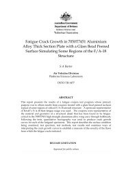
DSTO–TN–0640ZmeridianPrimeYXEquatorFigure 1: The Earth-Centred, Earth-Fixed frame can take a set of cartesianaxes X, Y, Z with their origin at Earth’s centre. The X-axis points to the0 ◦ latitude, 0 ◦ longitude point. The Y -axis points to 0 ◦ latitude, 90 ◦ longitude.The Z-axis points to 90 ◦ latitude, along Earth’s axis of rotation.Earth’s surface is taken to be an oblate spheroid, i.e. having circular crosssection at all latitudes, and a constant elliptical cross section through anymeridian2.1 ECEF: the Earth-Centred, Earth-Fixed FrameFor most situations, and certainly all in this report, the Earth-Centred, Earth-Fixed Frame(ECEF) is a very useful stage on which to play out all scenarios, from the point of viewof calculating orientations and directions for aircraft with global movements. All manipulationsof numbers are done by using cartesian coordinate axes that are fixed in theECEF.The axes of the ECEF are right handed and have their origin at the centre of Earth,being fixed to its body: they rotate with it. They are quite adequate for describingsituations on Earth, but are not so useful for describing satellite motion, such as scenariosthat involve the GPS satellite system. The reason is because the ECEF frame is not quiteinertial: because of its rotation, Newton’s laws don’t quite hold in it (unless we introducecomplicated centrifugal and Coriolis forces), which means that satellite motion can be verycomplicated in the ECEF’s coordinates. For such motion, a more encompassing frame tiedto the fixed stars is used, but we won’t need such a one in this report.The ECEF has two common coordinate systems: a polar-type “latitude–longitude–height” called geodetic coordinates, and the simpler three cartesian axes X,Y,Z that areshown in Figure 1. Global positions are often given in lat–long–height coordinates, butsince X,Y,Z are far easier to work with, we’ll convert all lat–long–height to X,Y,Z. A shapefor Earth commonly used in calculations is the oblate spheroid specified by the WorldGeodetic System 1984 standard (WGS-84), which has a circular cross section at any givenlatitude, and whose cross section through any meridian is an ellipse, having identical axeslengths for all longitudes. These axes lengths are, by definition,Semi-major: a = 6,378,137 mSemi-minor: b = 6,356,752.3142 m. (2.1)2

DSTO–TN–0640These numbers—especially b with its extra decimal places—might appear to be specifyinga completely over-optimistic accuracy; but they are simply a combination of measurementand best fit to an ellipse, and so they just define WGS-84.Any point has latitude α, longitude ω, and height h in this report. (There is no standardconvention for latitude and longitude angles, so we have used the second letter of each word[“a” and “o”] and written them with Greek letters.) The latitude and longitude are shownin Figure 2, while the height of the point is the distance above the reference spheroid,i.e. along a line normal to it, not along a line extending from Earth’s centre.The reason the latitude is defined with reference to the local normal and not Earth’scentre, is because by using the local normal, we can be sure that if two points on the samemeridian have latitudes of say 10 ◦ and 50 ◦ , then the normal line (i.e. the local vertical) isguaranteed to rotate through 40 ◦ when passing from one to the other. So it’s very easy tocompute how the vertical changes over Earth’s surface, and this would not be the case iflatitude was measured relative to Earth’s centre.Given lat-long-height values for any point, the corresponding X, Y, Z values are givenin terms of a and b by:X =⎛⎝√a⎞+ h⎠ cos α cos ω ,cos 2 α + b2 sin 2 αa 2⎛⎞Y = ⎝√a+ h⎠ cos α sin ω ,cos 2 α + b2 sin 2 αa 2⎛⎞Z = ⎝√b+ h⎠ sinα. (2.2)a 2cosb 2 α + sin 2 α2The inverse transformation process is lengthier. Finding the longitude is the easiest part:cos ω =X√X 2 + Y , sinω = Y√ 2 X 2 + Y , (2.3)2so that for example in C and Matlab, ω can be found by using the single commandomega = atan2(Y,X). (Note that in Excel, the same function atan2 has its argumentsreversed, so would be atan2(X,Y) here.)Latitude is more difficult, but can be calculated iteratively with reasonable ease. Beginwith a first estimate( ) aα ≃ tan −1 2Z√ , (2.4)X 2 + Y 2b 2where e.g. Matlab’s atan function will suffice (atan2 is not necessary), and then iterateto refine this estimate using⎛⎞α = tan −1 ⎝a 2 sin 2 α( √X √ ⎠. (2.5)b 2 sinαcos α + 2 + Y 2 sinα − Z cos α)a 2 cos 2 α + b 2 sin 2 α(This will fail if Z = 0, but then α = 0 trivially anyway.) This expression for α convergesvery quickly; in fact about five decimal places of precision is obtained by only using the3

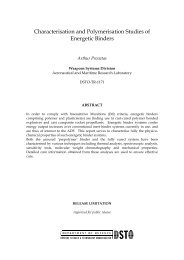
DSTO–TN–0640ZNorthEastωDownαYXFigure 2: A plane tangent to Earth’s hypothetical spheroidal surface containsthe local East and North directions, which set those axes for the North–East–Down frame. The Down axis is normal to this plane. The latitude α ofthe point at the origin of the NED frame is set by the angle at which theDown axis intercepts Earth’s equatorial plane. Because Earth is modelledas an oblate spheroid, the Down axis only points toward its centre when theNED origin is on the equator or at the poles. An alternative set of axes isEast–North–Upfirst estimate (2.4) and not even iterating at all. Finally, after an acceptable estimate of αhas been obtained, the height is calculated:h =√X 2 + Y 2cos α−a 2√a 2 cos 2 α + b 2 sin 2 α . (2.6)2.2 The Local Geographic FrameAt any point on Earth’s surface, the local geographic frame is defined by the almost flatground and the vertical direction, and is relevant because it is the basic reference theaircraft flies against, defining straight and level flight and of course the direction of down.This is an intuitive frame for any scenario whose total extent is no more than some tensof kilometres.Two coordinate systems are used: both cartesian with their origins at the point inquestion. In the North–East–Down or NED frame, shown in Figure 2, the local directionsof north, east, and down define a right-handed set of three axes. An alternative choiceof cartesian axes is the local East–North–Up set (ENU). In both axes sets, the north andeast directions define a plane tangent to Earth’s surface. At any point, north points alongthe local meridian, while east points along the local small circle of constant latitude.The up/down or vertical direction is perpendicular to this plane. In general, the verticaldirection does not intersect Earth’s centre. Rather, it makes an angle of the latitude withthe equatorial plane, shown as the angle α in Figure 2.4

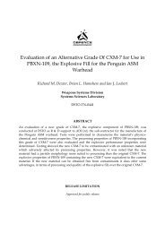
DSTO–TN–0640y+(Pitch axis)+x(Roll axis)+z(Yaw axis)Figure 3: The x, y, z axes of the aircraft’s own frame. These are axes aboutwhich the aircraft rolls (x), pitches (y), and yaws (z), where the direction ofpositive rotation for each is given by the right hand rule2.3 An Aircraft’s Own FrameThe aircraft itself has its own frame described by a set of axes at rest relative to it, asshown in Figure 3. Conventionally the x-axis points forward along the nose, the y-axispoints out along the starboard wing, and the z-axis points down. The x, y, z axes of anaircraft flying straight and level due north will match the local NED axes (i.e. x = north,y = east, z = down).3 The Basic Tool: Vector RotationsSwitching between frames involves rotating vectors about specified axes, and just howto rotate vectors forms one of the core tools described in this report. In this section wepresent the main formula for doing this. Surprisingly, this matrix formula for a generalrotation in three dimensions can be hard to find in textbooks. Before giving the generalexpression, we’ll start from more basic ideas.3.1 Matrix Representation of an OrientationHow can we represent the orientation of a body in three dimensions? We can only doit in a relative way, by specifying how the body has been moved from some initial, orbase, position. Suppose that the body is not translated, but its orientation is changed insome arbitrary way from this base position. Locate the body relative to the unmovingbasis vectors, and imagine the body taking a copy of each basis vector along with it as itchanges orientation. What are these new vectors? If the old ones are⎡ ⎤ ⎡ ⎤ ⎡ ⎤1i ≡ ⎣0⎦ ,00j ≡ ⎣1⎦ ,00k ≡ ⎣0⎦ , (3.1)15

DSTO–TN–0640then suppose they are transformed into column vectors i ′ , j ′ , k ′ . In that case, the changein orientation can be described by the matrixA = [ i ′ j ′ k ′] . (3.2)in the sense that this multiplies i to give i ′ , and similarly j, k. This expression is useful inthat it gives the matrix that transforms an initial orientation to a final one immediately,without our needing to work out how the final orientation was produced.If the body is rigid, then the linearity of matrix multiplication ensures that this matrixwill describe the orientation of the whole body. That is, any other point in the basepositionedbody that’s described by a certain linear combination of the basis vectors i, j, k,will be described by the same linear combination of the new basis vectors i ′ , j ′ , k ′ in thenew orientation. So the matrix A multiplies any vector to produce its orientated form.The same result holds for the more trivial two dimensional case, where we rotate allvectors through θ in the xy plane, positively about the z-axis. The basis vectors thenmap as:[ 1i = −→0][ ] [ cos θ= i ′ 0, j = −→sinθ 1][ ] − sinθ= j ′ , (3.3)cos θgiving the familiar rotation matrixA = [ [ ]i ′ j ′] cos θ − sinθ=. (3.4)sinθ cos θ3.2 Euler AnglesIn two dimensions the above transformation cannot help but be a rotation, but in threedimensions it’s not explicitly so; it simply produces a final orientation given some initialorientation. Nevertheless, it can be shown to be producible by just one rotation aroundsome axis, where that axis needn’t be any of the x, y, or z axes (and in general won’t be).This is known as Euler’s theorem.The literature actually spends more time on the fact that the final orientation can beproduced by successive rotations around the space-fixed x, y, z axes, through what areknown as Euler angles. There are many different conventions for specifying Euler angles,but in any of them, three angles are required to describe a general change in orientation.Some authors leave one axis out and repeat another, so that the orientations are performedaround, for example, the x-axis, then y-axis, then x-axis again (and all similar choices ofthree distinct rotations will also work, such as z, y, z etc.—but not e.g. z, y, y, since thisis really only two distinct rotations). Some rotate around the x-axis, then the new y-axis(better called y ′ ), then the new x-axis (now called x ′ ), although this can be shown toreduce to a similar expression involving the same angles but in a different order, aroundthe space-fixed x, y, x axes. The possibilities are many and confusing.Two Euler angles are also used in the field of aircraft tracking, where for example aradar might be used to follow the motion of an aircraft. At any moment, the aircraft’sposition can be specified by azimuthal and elevation angles, as if we were using a telescopewith a standard tripod to sight the aircraft. When the aircraft is nearly overhead, thetelescope becomes difficult to move easily, because the closer we come to pointing it at6

DSTO–TN–0640the zenith, the more its azimuthal motion (motion about the vertical axis) constricts itstube to making smaller movements. This means that small movements around the zenithtranslate to large changes in the azimuthal angle, which can be difficult to achieve evenly.Mechanically this constricted movement is called gimbal lock. In using these two anglesto track an aircraft, rapid changes in azimuth can be difficult to model in any numericalalgorithm, and the term gimbal lock has also come to be applied to numerical difficulties.The result is that it has given Euler angles a bad name. But the problem is purely one ofnumerical stability; there’s nothing wrong with using the two Euler angles in principle.This constriction of motion about one axis also causes mechanical problems with somegyroscopes. To picture why this might be, imagine a very simple (and not very useful)example of an inertial navigation system: a horizontal spinning flywheel carried on a yokeattached to hinges at the end of each wingtip, and held underneath the aircraft while itflies straight and level. The flywheel’s axis determines the up/down direction used bythe autopilot to help keep the aircraft on course. The aircraft can pitch up and downand yaw in the local north–east plane without affecting the flywheel’s motion. But if thehuman pilot tries to roll, the flywheel will be forced out of its spin plane. In such an event,the inertial navigation system will be fooled into believing that the aircraft has begunto develop some serious instabilities which it will try to correct, with perhaps disastrousconsequences. While this is a big simplification of a real system, it does encapsulate theproblem that can happen with a real gyroscope when the plane’s attitude reaches someextreme position.One way of avoiding numerical instabilities in tracking algorithms is to use Euler’stheorem, which does away with having to use three angles around the three fixed axes. Soit is that our matrix A in (3.2) describes this rotation. In principle it should be sufficientfor all purposes, although in practice its nine entries can require a powerful ability fornumber crunching, especially when used to describe motions where the orientation anglesare changing with time.3.3 The Workhorse: Rotating in Three DimensionsThe matrix A in (3.2) describes the rotation that changes a body’s orientation, providedwe know how the basis vectors change. But usually we are not given the final positionof those vectors. In general, we need to be able to rotate an arbitrary vector around anarbitrary axis, and this is a slightly different task to be done.This rotation can be done by multiplying the vector by a matrix R n (θ) that we writedown in this section. R n (θ) specifies a right-handed rotation through some angle θ aboutan axis aligned with a unit vector n. (Requiring n to have unit length makes the expressionssimpler.) It rotates the vector x to give x ′ , as shown in Figure 4:Write the unit vector that points along the axis of rotation asx ′ = R n (θ) x. (3.5)⎡ ⎤n 1n = ⎣n 2⎦ , (3.6)n 37

DSTO–TN–0640nθx ′xFigure 4: The matrix R n (θ) rotates x in a right-handed sense around theunit vector n by an angle θ to produce x ′ . That is, x ′ = R n (θ) xwhere n can point in either direction along the axis, but changing the choice of that directionwill change the sign required for the rotation angle θ, since the rotation matrix R n (θ)obeys the right hand rule for rotation. The rotation matrix can be written in the followingway, which is the main equation of this report:⎡⎤⎡⎤n 2 1 n 1 n 2 n 1 n 3R n (θ) = (1 − cos θ) ⎣n 2 n 1 n 2 2 n 2 n 3⎦ + cos θ I 3 + sinθ ⎣n 3 n 1 n 3 n 2 n 2 30 −n 3 n 2n 3 0 −n 1⎦−n 2 n 1 0= (1 − cos θ) nn t + cos θ I 3 + sin θ n × , (3.7)where n t is the transpose of n, I 3 is the 3 × 3 identity matrix, and⎡⎤0 −n 3 n 2n × ≡ ⎣ n 3 0 −n 1⎦ , (3.8)−n 2 n 1 0so-named becausen × x = n × x, (3.9)(with the n written nonbold to emphasise its matrix form). The rotation matrix R n (θ)is called orthogonal, by which is meant RR t = R t R = 1, and as well its determinant isalways 1. Equation (3.7) will be used repeatedly in this report to break more complicatedprocedures up into single rotations that are easy to visualise and easy to code. It is, infact, the central equation of the whole of rotation theory.Example of the use of (3.7): Rotate the vector (2, 0, 0) by 90 ◦ about the y-axis.What vector results? The required rotation matrix is R y (90 ◦ ) (where by the subscript yis meant n = (0, 1, 0) t ). Equation (3.7) gives it as⎡ ⎤ ⎡ ⎤ ⎡ ⎤0R y (90 ◦ ) = nn t + n × = ⎣1⎦ [ 0 1 0 ] + ⎣00 0 10 0 0⎦ = ⎣−1 0 00 0 10 1 0⎦ . (3.10)−1 0 0(Actually, in this simple example we can calculate R y (90 ◦ ) alternatively using (3.2). Simplynote that the basis vectors rotate as⎡ ⎤ ⎡ ⎤ ⎡ ⎤ ⎡ ⎤ ⎡ ⎤ ⎡ ⎤1 0 0 0 0 1⎣0⎦ −→ ⎣ 0⎦ , ⎣1⎦ −→ ⎣1⎦ , ⎣0⎦ −→ ⎣0⎦ , (3.11)0 −1 0 0 1 08

DSTO–TN–0640so that (3.2) yields R y (90 ◦ ) trivially.) The required rotated vector is thenas expected.⎡ ⎤ ⎡ ⎤⎡⎤ ⎡ ⎤2 0 0 1 2 0R y (90 ◦ ) ⎣0⎦ = ⎣ 0 1 0⎦⎣0⎦ = ⎣ 0⎦ , (3.12)0 −1 0 0 0 −2An example of combining two rotations is given in Appendix A. As stated by Euler’stheorem, the effect of these is just one rotation, although the values of the resultingequivalent axis and angle turned through are not obvious at all from the original two axesand angles.The rows of a rotation matrix will gradually lose their mutual orthonormality becauseof rounding errors under repeated iterations in a computer programme. This wanderingcan be kept in check by periodically re-orthogonalising, accomplished byR → R ( R t R ) −1/2 . (3.13)Rotation Order and its Possible Blind ApplicationSince matrix multiplication is not commutative, two rotations are also not in general commutative:the result depends on the order in which they are done. However, infinitesimalrotations are commutative. This fact can be used to our advantage when writing computercode that takes inputs from a joystick, in order to rotate a scene (say, in a flightsimulator). The pilot might induce both a pitch and a roll, but only by applying each ofthese in tiny increments will the software successfully reproduce the effect that the pilotwants.Nevertheless, it’s possible to go to an extreme of demanding a set rotation order thatdoes not mimic what the user of a software package wants, but that does do somethinghighly misleading. In fact, a search through the internet shows that this mistake seems tobe a classic of computer graphics programming, and has caused some in that community todistrust the mathematics of rotation. An example of this incorrect application of rotationsis discussed in Appendix C.3.4 Rotating using QuaternionsAlthough the rotation matrix R n (θ) has nine entries, it’s really only built from three numbers:the angle θ turned through, and any two components of n; the third component of nis then implied, since n has unit length. Using R n (θ) can be computationally inefficient,since not only do all nine components need to be manipulated, but if the matrix is appliedwithin a loop, perhaps thousands of times, numerical inaccuracies can degrade itsorthogonality. That is, its rows (or equivalently columns) will slowly lose their mutualorthonormality. It can certainly be periodically re-orthogonalised after an appropriatenumber of iterations, as shown in (3.13). Nevertheless, the question arises as to whetherany way exists of rendering the matrix down to its basic three numbers, and perhapseliminating some of the numerical complexity in the process.9

DSTO–TN–0640We are always free to construct any quantity from those three numbers. For instance wecould specify a rotation through θ around (n 1 , n 2 , n 3 ) by a new object written as (θ, n 1 , n 2 ).This is very concise, but the catch is that we would also have to define how this objectacts on a vector to rotate it. The result is not anything simple, so we gain nothing bydoing this.But all is not lost. If we allow a little more complexity, and construct a new object Q n (θ)from θ, n 1 , n 2 , n 3 along with a sine and cosine, then this turns out to be simple enough tooffset the more complicated way it has to interact with vectors. Here n is taken to be theunit row vector (n 1 , n 2 , n 3 ):(Q n (θ) ≡ cos θ 2 , nsin θ ). (3.14)2This new object Q n (θ) is called a rotation quaternion. More general quaternions (not forrotating) are composed of a number and a vector: (a 0 , a). Two quaternions multiply inthe following way:(a 0 , a)(b 0 , b) ≡ (a 0 b 0 − a·b, a 0 b + b 0 a + a×b) , (3.15)so that the squared length of a quaternion is defined to be (in analogy to the length of avector):∣∣(a 0 , a) ∣ 2 ≡ a 2 0 + |a| 2 . (3.16)We can see straight away that a rotation quaternion Q n (θ) has unit length, which is theequivalent property of rotation quaternions as orthogonality and a unit determinant is ofrotation matrices.Using rotation quaternions, a row vector x can be rotated through an angle θ arounda unit vector n by applying a double multiplication:(0, x ′ ) = Q n (θ) (0, x)Q −n (θ), (3.17)where quaternion multiplication is associative, so either product can be done first. Asan example, in (3.12) we used a matrix to rotate (2, 0, 0) by 90 ◦ about the y-axis togive (0, 0, −2). Contrast the matrix approach with the quaternion approach:(0, x ′ ) =( )1 1 √2 , √ (0, 1, 0) 2(0, 2, 0, 0)= (1, 0, 1, 0)(0, 1, 0, 0)(1, 0, −1, 0)so that the result is (0, 0, −2) as expected.( 1 √2 , √ −1 )(0, 1, 0) 2= (0, 0, 0, −2), (3.18)Combining two rotations using quaternions is straightforward. Just as a matrix rotationR 1 followed by R 2 is equivalent to a single matrix rotation R 2 R 1 , a quaternionrotation Q 1 followed by Q 2 is equivalent to a single quaternion rotation Q 2 Q 1 .Finally, just as a rotation matrix will slowly lose orthogonality under repeated iterationsin a software routine, so a rotation quaternion’s length will slowly wander from one in thesame circumstances. It can be periodically reset by dividing each of the quaternion’s fourelements by the length calculated from (3.16), which is a very much simpler task thanre-orthogonalising a matrix in (3.13).10

DSTO–TN–0640Matrix Cost versus Quaternion CostHow expensive is using matrices as opposed to using quaternions? While (3.18) mightlook succinct, it does hide some effort, especially in the two cross products that have beendone. In Table 1 we give simple counts of operations required to rotate a vector, if donewith pen and paper. No allowance for numerical optimisation is made since that forms afield in itself. It can be seen that quaternions are easier to build, while matrices are easierto use; thus, depending on the application, it can be useful to convert between the twosubject to how much of each process needs to be done.Table 1: First-principles computation costs of matrices and quaternions, forthe build and one use of each. The numbers shown are not optimisedMatrixQuaternionBuild 2 trigonometric functions, 2 trigonometric functions,using (3.7) and (3.14): 10 additions, no additions,21 multiplications. 4 multiplications.One rotation 6 additions, 24 additions,using (3.5) and (3.15, 3.17): 9 multiplications. 30 multiplications.Multiplication 27 multiplications, 16 multiplications,18 additions. 12 additions.The benefit of using quaternions for iterative calculations is that the resetting of aquaternion’s length to 1 requires a simple division by its length, calculated from (3.16).On the other hand, re-orthogonalising a matrix from (3.13) is a much more complicatedaffair that involves the lengthy procedure of matrix diagonalisation. Although there isroom for optimisation in this process, it cannot compete with quaternion normalisation forsimplicity. How often such a resetting or re-orthogonalising needs to be done is presumablya function of the numerical complexity of the problem being tackled.In fact, it might be thought that rather than use the expensive (3.13) to re-orthogonalisethe matrix, that a better approach would be to convert the matrix to a quaternion, normalisethat, and then convert back to a matrix. This can be done using the analysis ofAppendix A, by applying (A1) to produce the angle and axis from the matrix, that arethen used to build the quaternion via (3.14), which is then normalised and converted backto a matrix using (3.7). But whether this is really viable might depend on the numericalaccuracy of the software. As it is, (A1) only samples the matrix’s three diagonal elementsto calculate the angle θ, perhaps producing too inaccurate a result to be used in buildingthe quaternion. The quaternion could be produced by using all of the matrix elements; butit’s not clear what work has been done in this area for doing this efficiently and accurately.4 Rotating Axes to Change CoordinatesThe building block that allows all manner of aerospace re-orientations to be done, forvarious pitches, rolls, yaws, changes of latitude/longitude, and local geographic frames, is11

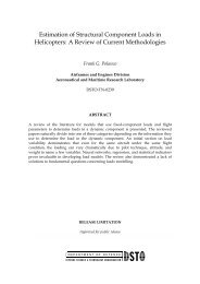
DSTO–TN–0640ZNDEN 0E 0D 0 N 1E 1ωαYXD 1Figure 5: Constructing local north–east–down axes N, E, D at a given pointof known latitude and longitude. Start with the three vectors N 0 , E 0 , D 0 .Construct the intermediate set N 1 , E 1 , D 1 by rotating the original setthrough the longitude ω about N 0 . Then rotate N 1 , E 1 , D 1 about −E 1 by thelatitude α, according to the right hand rule, to give the final set N, E, D. Orequivalently, rotate the intermediate set about E 1 through minus the latitude.The resulting vectors are the local north–east–down axesthe act of rotating each of the vectors that represent the axes of some frame.There are two basic tasks to consider in this type of aerospace calculation. First, givena place on Earth (usually in lat–long–height coordinates), we need to construct the localgeographic frame’s axes, such as NED. Second, an aircraft can be introduced into thisNED frame, and its orientation found relative to that frame.4.1 Constructing NED Axes for the Local Geographic FrameGiven the lat–long–height of a place on or near Earth, the first thing we wish to do is findthe local NED axes. The technique used is the primary one of this report. We build aninitial set of NED axes in a place where it’s simple to determine them, and then we rotatethese around to the required place.The simplest place to construct an initial set of NED axes is on the junction of theEquator and the prime meridian, since this has a latitude and longitude of α = ω = 0 ◦ .Represent each axis by a unit vector in the ECEF frame, which all calculations are beingdone within:⎡ ⎤0⎡ ⎤0⎡ ⎤−1N 0 = ⎣0⎦ , E 0 = ⎣1⎦ , D 0 = ⎣ 0⎦ . (4.1)1 0 0The scenario is shown in Figure 5. Now rotate each of the N 0 , E 0 , D 0 vectors in two steps.12

DSTO–TN–0640The first rotation is about the N 0 vector by the longitude ω, taking care to realise thatthe rotation matrix will obey the right hand rule. This rotation creates an intermediatetriplet of vectors, taking N 0 →N 1 , E 0 →E 1 , D 0 →D 1 . (Of course, N 1 = N 0 , but forclarity we keep each triplet together notationally.)Now rotate each of the intermediate set by the latitude α about −E 1 ; again we’ve beencareful to note the use of the right hand rule, so need to specify the axis of rotation as −E 1 .(We can certainly use +E 1 , but will have to rotate by −α about this. The rotation matrixor quaternion will be unchanged.) Because the original N 0 , E 0 , D 0 vectors each haveunit length, they automatically satisfy the requirement for the axis vector n to be of unitlength in (3.7). Notice that the clever way that latitude has been defined means we needn’tworry that Earth’s shape is not spherical; two places separated by say 50 ◦ latitude on thesame meridian will certainly have a 50 ◦ angle between their North vectors, and a 50 ◦ anglebetween their Down vectors.The sequence of steps is:N 1 = R N0(ω)N 0 = N 0E 1 = R N0(ω)E 0D 1 = R N0(ω)D 0N = R −E1(α)N 1E = R −E1(α)E 1 = E 1D = R −E1(α)D 1 . (4.2)The resulting vectors N, E, D are the local north–east–down axes, and can be used forfurther calculations. In the interest of pedagogy, we have made the steps as alike aspossible, but in practice they can be heavily reduced toE = R N0(ω)E 0N = R −E(α)N 0D = N × E . (4.3)This reduction is purely a question of pedagogy versus computational speed. Equations(4.2) allow for a step by step follow-through of the process, which is useful forwriting transparent computer code or debugging in more complicated situations wheremore than two rotations need to be performed. In this two-rotation case, it’s certainly notdifficult to use (4.3) without having to think along the lines of (4.2) at all. But situationsrequiring more than two rotations will not be so easily abbreviated.The following example draws many of these ideas together.Example: If we are in Adelaide and Earth is transparent, what is the compass bearing ofBrussels if we are looking straight at it through Earth?We’ll calculate ECEF position vectors of both Adelaide and Brussels, subtracting onefrom the other to find the position vector of Brussels relative to Adelaide, and then expressthis in the local NED axes at Adelaide using dot products. It’s helpful to write the vectorsin the following way, where A = Adelaide, B = Brussels, and C = some other useful point.13

DSTO–TN–0640The vector giving the position of B relative to A can be written r B←A, and the followingare all true in general, as well as being useful for writing down vector relationships withoutneeding to draw pictures:r B←A= −r A←Br B←A= r B←C− r A←Cr B←A= r B←C+ r C←A(4.4)The cities’ positions are:Adelaide: latitude α = −34.9 ◦ , longitude ω = 138.5 ◦ ,Brussels: latitude α = 50.8 ◦ , longitude ω = 4.3 ◦ .Use (2.2) to find the position of each city relative to Earth’s centre (which is exactly whatthe ECEF coordinates specify): set C = Earth’s centre.⎡ ⎤⎡ ⎤−3.924.03r A←C= ⎣ 3.47⎦ × 10 6 metres, r B←C= ⎣0.30⎦ × 10 6 metres. (4.5)−3.634.92The position of Brussels relative to Adelaide is then⎡ ⎤7.95r B←A= r B←C− r A←C= ⎣−3.17⎦ × 10 6 metres. (4.6)8.55This vector is still an ECEF vector, although we can consider it to start at Adelaide andpoint to Brussels. To calculate the bearing of Brussels as seen from Adelaide, we needto get the local north and east components of r B←A. To do this, we’ll first calculateAdelaide’s local north, east, and down axis vectors, labelled N, E, D in Figure 5, all inECEF coordinates, using (4.2). For this we need R N0(ω), constructed from (3.7):⎡ ⎤⎡⎤0−0.74896 −0.66262 0N 0 = ⎣0⎦ , ω = 138.5 ◦ , R N0(ω) ≃ ⎣ 0.66262 −0.74896 0⎦ . (4.7)10 0 1This R N0(ω) then acts in (4.2) to produce N 1 , E 1 , D 1 . We then use −E 1 to construct thenext rotation matrix R −E1(α), which finally produces the N, E, D. The steps are easy toprogramme and are omitted; the resulting axes are⎡ ⎤ ⎡ ⎤ ⎡ ⎤−0.429−0.663N = ⎣ 0.379⎦ , E = ⎣−0.749⎦ , D = ⎣0.820 00.614−0.543⎦ . (4.8)0.572The bearing of Brussels is calculated by projecting r B←Ainto the local north–eastplane. The projection can be visualised as an arrow drawn on the ground, so that itsangle from north is the required bearing. The projection in the local north–east plane issimply given by the components of r B←Aon the local north and east axes. These are dotproducts:North component = r B←A·N = 2.4035 × 10 6 metres,East component = r B←A·E = −2.8958 × 10 6 metres. (4.9)14

DSTO–TN–0640(Note that these equations assume the axis vectors N, E have unit length; another reasonto prefer unit length axis vectors from the start.) The units here are immaterial; the onlything that matters is the ratio of the components, so that Brussels’ bearing is360 ◦ −1 2.8958− tan2.4035 ≃ 310◦ , (4.10)or roughly north-west. Apart from the initial change of variables in (2.2), this wholecalculation has been accomplished using just rotations and dot products. We could ofcourse have streamlined it using (4.3) as well as omitting the calculation of the local Downvector D, but the point here is pedagogy, not efficiency.4.2 The World as Seen by a PilotSometimes we wish to know the appearance of a scenario as seen by the pilot. For exampleif an aircraft is flying straight and level, and then executes a series of yaws, pitches, androlls, where will the compass directions lie, and where will “up/down” be? If an aircraft isalongside but 200 m higher, where will this aircraft be seen to lie from the confines of thecockpit?These questions are answered by rotating vectors. To determine where the compassdirections are, we need to know where the aircraft is headed before it turns. Thesedirections are only really well defined near Earth’s surface, and in this case, each ofthem can be considered as vectors emanating from the cockpit itself, described in theaircraft’s frame. For example, Fig. 3 shows that if the aircraft is flying straight and levelnorth-east, then the north direction vector will have coordinates in the aircraft’s frameof (x, y, z) = (1/ √ 2, −1/ √ 2, 0).Example: This involves large distances just to ensure the method is well understood. Supposewe are flying north-east over Adelaide, pitched up at 20 ◦ at an altitude of 30,000m.We sight an aircraft flying over Sydney at the same altitude. In which direction in thecockpit must we look to see that aircraft?As usual, work in the ECEF. Call the other aircraft “them”, and construct a vectorpointing from our location to them. This is the vector of them relative to us, or r them←us.We require the components of this vector in the aircraft frame. These components aregiven by dotting r them←uswith the three vectors describing each of the aircraft’s axes.The axes are x, y, z in Fig. 3, and we’ll call the vectors along each one x, y, z, respectively.So we need to findr them←us·x , r them←us·y , r them←us·z . (4.11)The vector r them←usis found simply by referring everything to the centre C of Earth,which implies using the ECEF:r them←us= r them←C− r us←C. (4.12)The vector r them←Cis just their position in the ECEF, and r us←Cis our own position inthe ECEF. These positions are given by applying (2.2) to Adelaide’s and Sydney’s latitudeand longitude, together with the given heights both of 30,000 m. The two cities lie at:Adelaide: latitude α = −34.9 ◦ , longitude ω = 138.5 ◦ ,Sydney: latitude α = −33.9 ◦ , longitude ω = 151.2 ◦ .15

DSTO–TN–0640Equation (2.2) together with the appropriate heights then gives approximately:⎡ ⎤−4.67⎡ ⎤−3.94r them←C= ⎣ 2.57⎦ × 10 6 metres, r us←C= ⎣ 3.49⎦ × 10 6 metres. (4.13)−3.55−3.65Hence⎡ ⎤−7.25r them←us= r them←C− r us←C= ⎣−9.21⎦ × 10 5 metres. (4.14)0.92Now we need to find x, y, z at our location. First we find the local north, east, anddown vectors N, E, D by (4.2) or (4.3), where the heights play no part in the calculation.These were given in (4.8). These vectors must be rotated to produce our own aircraftaxes. First, place our aircraft in the local NED frame flying north, straight and level. Itsaircraft axes then match the local NED axes:x 0 = N , y 0 = E , z 0 = D . (4.15)Next rotate the aircraft axes around z 0 by 45 ◦ , and then rotate 20 ◦ around the new y-axis y 1 , taking care to get the angle signs right by way of the right hand rule for rotation.The sequence is:x 1 = R z0 (45 ◦ )x 0y 1 = R z0 (45 ◦ )y 0z 1 = R z0 (45 ◦ )z 0 = z 0x = R y1 (20 ◦ )x 1y = R y1 (20 ◦ )y 1 = y 1z = R y1 (20 ◦ )z 1 . (4.16)The final vectors are approximately⎡ ⎤−0.94⎡ ⎤−0.17⎡ ⎤0.31x = ⎣−0.06⎦ , y = ⎣−0.80⎦ , z = ⎣−0.60⎦ . (4.17)0.35−0.58 0.74Dotting these with r them←usin (4.11) gives the set of components we require, so that theother aircraft turns out to have coordinates (765, 802, 393) km in the frame of our aircraft.(Note that these numbers result from keeping more significant figures than are shown inthe numbers above.) As a simple check, the length of this vector should be the distanceof the aircraft:distance of aircraft = √ 765 2 + 802 2 + 393 2 km ≃ 1176 km, (4.18)which is reasonable. To actually sight the aircraft, we first need to turn our head to ourright by approximately tan−1 802765 , or 46◦ . Again this makes sense, since the aircraft isapproximately due east and we are already flying north-east. After having turned ourhead through 46 ◦ , we need to turn it downwards by tan−1 √ 393765 2 +802 2, or about 20◦ .16

DSTO–TN–06404.3 ECEF Coordinates and Heading-Pitch-Roll ConversionTypically, simulation software will store object locations in lat–long–height, as well asorientations in a heading–pitch–roll format: three Euler angles with respect to its localNED frame. “Heading” here means where the aircraft’s x-axis points, not the direction inwhich it’s actually travelling over the ground, which is called its track. Note that headingis not the same as yaw. Yaw is the angle between an aircraft’s heading (into wind, not overground), and the direction in which its nose points. An aircraft usually flies with no yaw,meaning that it’s pointing exactly into the oncoming air flow; the air flow is approachingdirectly over its nose. We, together with software packages, are really assuming the aircraftis not yawed, which is a very normal way to fly. Only some extreme fliers will hold a yawafter finishing their turn.Despite lat–long–height and heading–pitch–roll formats, an IEEE standard specifiesthat in order to communicate location–orientation between different machines in a distributedinteractive simulation (DIS) environment, XYZ coordinates be used, along witha different set of Euler rotations. The DIS standard says that three Euler rotations areimplemented by first rotating around the z-axis, then around the new y-axis, and finallyaround the newest x-axis. This order is useful because it corresponds to physical situations;for example, ones in which an aircraft might manoeuvre by changing its heading (about itsz-axis), then pitching (about its new y-axis), and finally rolling (about its newest x-axis).Proprietary software might well include routines to convert to and from these coordinates,but this software tends to be provided without source code and so generally is not portable.To aid in developing routines that use the DIS standard, this section describes how suchconversions can be done.The first set of DIS coordinates is the aircraft’s location in the XYZ coordinates of theECEF frame. The second set of coordinates is the set of three Euler angles that specifythe aircraft’s orientation by starting with its own axes coincident with the ECEF’s XYZaxes, and then rotating. The three rotations are by angle ψ around Z, then by θ aroundthe rotated Y , and finally by φ around the latest rotated X.After distribution, these numbers (X, Y, Z, ψ, θ, φ) might need to be converted back toa lat–long–height and an orientation with respect to the local NED axes.Converting the aircraft’s location to and fro between XYZ and lat–long–height wasdone in (2.2)–(2.6). The next task we’ll address is calculating the Euler angles ψ, θ, φ. Aswe’ll see in (4.30) ahead, it’s necessary to solve the problem for a general set of startingvectors, as opposed to X, Y , Z, so we’ll restate it using more general vectors. Supposewe have an orthonormal set of vectors (i.e. mutually orthogonal and all of unit length)x 0 , y 0 , z 0 . These are rotated by ψ about z 0 to give x 1 , y 1 , z 1 . These new are now rotatedby θ about y 1 to give x 2 , y 2 , z 2 . Finally, these latest are rotated by φ about x 2 to givex 3 , y 3 , z 3 :x 0 , y 0 , z 0R z0 (ψ)x 1 , y 1 , z 1R y1 (θ)x 2 , y 2 , z 2R x2 (φ)x 3 , y 3 , z 3 . (4.19)The question is: given x 0 , y 0 , z 0 and x 3 , y 3 , z 3 , what are ψ, θ, φ? These angles are asfollows. The angle ψ is given by projecting x 3 onto the x 0 y 0 plane, and is the angle ofthis projection from x 0 in the y 0 direction:xsinψ = √ 3·y 0(x3·x 0 ) 2 + (x 3·y 0 ) , cos ψ = x√ 3·x 02 (x3·x 0 ) 2 + (x 3·y 0 ) . (4.20) 2 17

DSTO–TN–0640Next, θ is the angle between x 3 and the projection just mentioned:sin θ = −x 3·z 0 , cos θ =Finally, φ is the angle from y 2 to y 3 in the z 2 direction:√(x 3·x 0 ) 2 + (x 3·y 0 ) 2 . (4.21)sin φ = y 3·z 2 , cos φ = y 3·y 2 . (4.22)Matlab code to calculate the first two of these angles would bepsi = atan2( dot(x3,y0), dot(x3,x0 );theta = atan2( -dot(x3,z0), sqrt((dot(x3,x0))^2 + (dot(x3,y0))^2) );For the last angle φ, we need y 2 and z 2 . These are given byAppropriate Matlab code is theny 2 = y 1 = R z0 (ψ)y 0 , z 2 = R y1 (θ)z 1 = R y1 (θ)z 0 . (4.23)phi = atan2( dot(y3,z2), dot(y3,y2) );The sequence of steps to convert to the six DIS numbers from a lat–long–height andheading–pitch–roll is as follows:1. Use (2.2) to convert lat–long–height (α, ω, h) to (X, Y, Z).2. Find the local NED axes as we did in Section 4.1. That is, start with X, Y , Z in theECEF frame and rotate, first through the longitude and then through the latitude,to give −D, E, N, respectively.3. Rotate the N, E, D vectors, first by the heading around D, then by the pitch aroundthe rotated E, and finally by the roll around the latest rotated N. The resultingvectors are, respectively, the aircraft’s local x, y, z axes (all in the ECEF frame).4. The angles ψ, θ, φ are calculated from (4.20, 4.21, 4.22), where we make the identificationsx 0 = X , y 0 = Y , z 0 = Z ,x 3 = x , y 3 = y , z 3 = z . (4.24)Example 1: An aircraft is flying 10,000m above Adelaide, heading south-east (with nowind component: the heading is taken as the direction in which the nose points), climbingat a 20 ◦ pitch, and holding a 30 ◦ roll. What are the two sets of triplets that the DISstandard requires to specify the aircraft’s locations and orientation?The location is found easily, by converting that aircraft’s lat–long–height at Adelaideto XYZ using (2.2):(X, Y, Z) = (−3.93, 3.48, −3.63) × 10 6 m. (4.25)18

DSTO–TN–0640The orientation vectors x, y, z are found by first calculating the local NED axes asvectors in the ECEF, and then rotating these by the relevant heading, pitch and roll.Some of this calculation has been done already in Section 4.1; the local NED axis vectorsare given there in (4.8). Using these, place the aircraft into the NED frame so that initiallyits x, y, z axes (i.e. x, y, z vectors) coincide with the N, E, D axes respectively, and nowrotate it as needed. So first setx 0 = N , y 0 = E , z 0 = D . (4.26)Now rotate x 0 , y 0 , z 0 each by 135 ◦ around z 0 (implementing the south-east heading),calling the result x 1 , y 1 , z 1 . Then rotate each of these by 20 ◦ around y 1 (implementing thepitch) to produce x 2 , y 2 , z 2 . Finally rotate each of these by 30 ◦ around x 2 (implementingthe roll) to produce x, y, z. Each of these rotations is easy to work out using the basicformula (3.7). The result is⎡ ⎤ ⎡ ⎤ ⎡ ⎤−0.366x = ⎣−0.564⎦ , y = ⎣−0.7410.928⎦ , z = ⎣−0.165−0.333Now calculate ψ, θ, φ from (4.20, 4.21, 4.22). To do this, set⎡ ⎤1x 0 = ⎣0⎦ ,⎡ ⎤0y 0 = ⎣1⎦ ,⎡ ⎤0z 0 = ⎣0⎦ ,0 0 1The resulting angles are0.065−0.809⎦ . (4.27)0.584x 3 = x , y 3 = y , z 3 = z . (4.28)ψ = −123.0 ◦ , θ = 47.8 ◦ , φ = −29.7 ◦ . (4.29)These, together with (X, Y, Z) given in (4.25), are the six numbers that the DIS standarduses to encode the aircraft’s position and orientation.Example 2: Convert back from X, Y, Z, ψ, θ, φ to lat–long–height/heading–pitch–roll.Again the location is found easily by applying (2.3)–(2.6). These equations return thelatitude α = −34.9 ◦ , longitude ω = 138.5 ◦ , and height 10,000m, as expected.To calculate the heading, pitch, and roll, realise that these are just the ψ, θ, φ, respectively,that are returned by step 4 above (4.24) when we make the following identifications:x 0 = N , y 0 = E , z 0 = D ,x 3 = x, y 3 = y , z 3 = z . (4.30)So we need to calculate N, E, D, which can be done as in Section 4.1, since we have justcalculated the latitude and longitude of the aircraft. These are given in (4.8).Next, the x, y, z are found by applying the three Euler rotations of ψ, θ, φ in theappropriate order, i.e. (4.19), to the ECEF’s basis vectors X, Y , Z. In other words, setx 0 , y 0 , z 0 in (4.19) to X, Y , Z. The three resulting vectors x 3 , y 3 , z 3 will be the requiredx, y, z.Finally, make the identifications of (4.30) to calculate ψ, θ, φ using (4.20, 4.21, 4.22),where the heading is ψ, the pitch is θ, and the roll is φ. As expected, we obtainheading = 135 ◦ , pitch = 20 ◦ , roll = 30 ◦ . (4.31)19

DSTO–TN–06405 Concluding RemarksAll of the commonly-needed techniques in three-dimensional rotations rely on our abilityto do two basic procedures:1. Rotate a vector about any axis whatsoever, and2. calculate components using dot products.These calculations need to be done in just one frame. The usual one is the ECEF, whichis good for all of the usual motions we associate with moving around Earth. (If we needto deal with satellites, a nonrotating frame is needed, such as one fixed to the stars.)Rotating about arbitrary axes and taking dot products within the ECEF is all that hasbeen done for the examples in this report.Rotations themselves can be carried out using matrices or quaternions. Both of theseare simply ways of writing down the three numbers needed to encode a rotation (anangle, and two numbers for the axis). The extra redundancy that matrices have overquaternions allows for simpler algebra when using matrices to analyse rotation on paper,but quaternions, being essentially pared-down versions of the rotation matrix, can be easierto prevent from degrading numerically inside a computer routine (but see the comment atthe end of Sect. 3.4). Performance questions like this are critical in that three-dimensionalmodels can have 10,000+ points to rotate at e.g. 30 frames per second.When solving a problem involving three-dimensional rotations, a good approach is tobreak the scenario down into its building block rotations and to handle each one separately,all within the ECEF. This step-by-step approach lends itself well to being modularised insoftware, and is what we have used repeatedly in this report.ReferencesMathematics essential to three-dimensional rotations is described in:Lyons, L., (1998) All You Wanted to Know About Mathematics But Were Afraid toAsk, Cambridge University PressVarious useful calculations involving GPS coordinates are contained in:Farrell, J., Barth, M. (1998), The Global Positioning System and Inertial Navigation,McGraw-Hill20

Appendix A Combining Two RotationsDSTO–TN–0640Earlier we said that two rotations will always combine to give a new rotation. This is ofcourse equivalent to multiplying the two rotation matrices or quaternions. But what isthe axis and angle of the new rotation? For example, suppose we rotate a vector twice:1. First rotate it by 90 ◦ around the x-axis (call the matrix R x and the quaternion Q x ).2. Then rotate it by 90 ◦ around the y-axis (call the matrix R y and the quaternion Q y ).What is the corresponding axis and angle of the combined rotation? We do this first usingmatrices and then with quaternions. It will be quite evident from the answer that tworotations generally don’t combine to give an obvious resulting angle and axis.Using MatricesThe combined matrix rotation is R y R x :⎡ ⎤ ⎡ ⎤1 1 0 01. R x : θ = 90 ◦ , n = ⎣0⎦, so R x = ⎣0 0 −1⎦0 0 1 0⎡ ⎤ ⎡ ⎤00 0 12. R y : θ = 90 ◦ , n = ⎣1⎦, so R y = ⎣ 0 1 0⎦0−1 0 0⎡ ⎤0 1 03. R y R x = ⎣ 0 0 −1⎦−1 0 0To find the single angle and axis of rotation that R y R x is equivalent to, we could compareeach element of R y R x with the general expression (3.7), but this is arduous. Much easieris to use (3.7) to write down two properties of the general rotation matrix, using its traceand its transpose:trR = 1 + 2 cos θR − R t = 2 sinθ n × . (A1)In that case, the combined rotation is around some unit vector n through angle θ, where⎡ ⎤0 1 11 + 2 cos θ = 0 , 2 sinθ n × = ⎣−10 −1⎦ .(A2)−1 1 0There appear to be two solutions for n and θ here, but they both represent the samerotation, so that we can always choose the unique positive value of θ together with itscorresponding n. In this case:θ = 120 ◦ , n = (1, 1, −1)/ √ 3 . (A3)21

DSTO–TN–0640Using QuaternionsThe necessary quaternions areQ x =Q y =()cos 45 ◦ , sin45 ◦ (1, 0, 0) = √ 1 (1, 1, 0, 0), 2()cos 45 ◦ , sin45 ◦ (0, 1, 0) = √ 1 (1, 0, 1, 0). 2(A4)The combined quaternion rotation is Q y Q x :Q y Q x = 1 2 (1, 0, 1, 0)(1, 1, 0, 0) = 1 (1, 1, 1, −1)(2√ ) ()1 3=2 , (1, 1, −1)√ = cos 60 ◦ (1, 1, −1), √ sin60 ◦ , (A5)2 3 3which is a rotation of 120 ◦ around (1, 1, −1)/ √ 3, just as we found in (A3).22

DSTO–TN–0640Appendix B xyz Eulers to Angle–Axis and ViceVersaIn this appendix we explain how to switch between an xyz Euler angle representation of arotation and the angle–axis representation characterised by a single rotation matrix R n (θ)or quaternion Q n (θ). This fixed-axis Euler representation differs to the DIS standarddiscussed in Section 4.3 because in this appendix, the axes rotated around are fixed inspace. Even so, the fixed-axis convention is also very commonly used.xyz Eulers to Angle–AxisSuppose a rotation is built of three Euler rotations: first by an angle α around the x-axis,then by β around y, then by γ around z. These join to give a single rotation of θ around n,given byR n (θ) = R z (γ)R y (β)R x (α),(B1)where the matrix R n (θ) encodes the whole rotation. If it’s necessary to know n and θexplicitly, they can be found by applying (A1).If the rotations are performed around new axes, then the calculation of the rotationmatrix is only a little more difficult. For example, suppose the second rotation is aroundthe new y-axis (called y ′ ), while the third is around the newest x, called x ′ :R n (θ) = R x ′(γ)R y ′(β)R x (α).(B2)The first rotation is done as usual: R x (α) rotates by α around (1, 0, 0). The second rotationis about the new y-axis, whose vector is⎡ ⎤0n 1 ≡ R x (α) ⎣1⎦ .(B3)0The last rotation, by γ, needs to be done around the new x-axis. This axis is representedby the vector⎡ ⎤1n 2 ≡ R n1 (β) ⎣0⎦ ,(B4)0so that the final rotation isR n (θ) = R n2 (γ)R n1 (β)R x (α).(B5)These calculations can of course also be done using quaternions, as detailed in Appendix A.23

DSTO–TN–0640xyz Angle–Axis to EulersIf the xyz rotation order of (B1) is used, a single rotation matrix R can be converted tothree rotations using the Euler angles α, β, γ, where s can be chosen as either +1 or −1:sinα =sR 32√1 − R231, cos α = sR 33√1 − R231sinβ = −R 31 ,√cos β = s 1 − R312sinγ =sR 21√1 − R231, cos γ = sR 11√1 − R231.(B6)The value of s is immaterial in the sense that either choice will give three angles thathave the same effect as the original rotation. Care is needed to avoid oversimplifying theseequations: we must remember that (B6) does not imply that e.g. α = tan −1 (R 32 /R 33 ),since the tan −1 function only gives angles in the range −90 ◦ → +90 ◦ . Nor does it implythat β must equal − sin −1 R 31 , because of a similar restriction on the sin −1 function.These equations can be implemented in Matlab using the code:alpha = atan2(s*R(3,2), s*R(3,3));beta = atan2(-R(3,1), s*sqrt(1-R(3,1)^2));gamma = atan2(s*R(2,1), s*R(1,1));24

DSTO–TN–0640Appendix C Confusing Euler Angle Orientationwith Incremental RotationAs we saw in Sect. 3.2, an object’s orientation can be specified by giving three Euler angles:angles through which the object can be turned in some preset order from a base position,which will result in the required orientation. This is useful and unambiguous, but it canlead to some confusion when implemented in an overly rigid way.The problem can be shown as follows. Suppose we have written computer code thatdraws some object, and supplies three graphical sliders that allow us to specify Euler anglesto change its orientation. We can alter any of the angles at any time, and the software willread the current values of the three angles, interpret them as Euler angles, and use themto rotate a preset base orientation of the object, first around the x-axis, then around y,and finally around z. The result is then displayed on the computer screen.When we start the programme, this graphical interface is always drawn with the threesliders each set to zero, and the object in its base position. If we alter the x-slider toread 10 ◦ and leave the other two sliders at zero, then the three angles are read by the software,and a rotation of R z (0)R y (0)R x (10 ◦ ) is applied. The object duly rotates around xby 10 ◦ . If we increase the x-slider to 15 ◦ , the software reads all the sliders again andapplies a rotation of R z (0)R y (0)R x (15 ◦ ) to the base orientation. The effect is that theobject is seen to rotate around x through a further 5 ◦ . We then set the x-slider back tozero, the three angles are again read, and the result is that the base orientation is rotatedby R z (0)R y (0)R x (0), or nothing at all. So changing the x-slider by itself rotates theobject about the x-axis, which is perfectly reasonable and expected.Similarly if we change only the y-slider, or only the z-slider, the same sort of intuitiveeffects happen. Setting the y-slider to 10 ◦ with the others at zero means that the softwarereads the three angles and applies a rotation of R z (0)R y (10 ◦ )R x (0) to the base orientation,so that the object rotates around y by 10 ◦ , and similarly it will revert to the base positionif we set the y-slider back to zero.Suppose we now change two of the angles; we’ll ignore the z-slider as it’s not needed tomake the following point. Start with all sliders at zero so that the object is drawn in thebase orientation. Then set the x-slider to 10 ◦ . The rotation is R y (0)R x (10 ◦ ), so the objectrotates around x by 10 ◦ . Now set the y-slider to 10 ◦ . The new rotation is R y (10 ◦ )R x (10 ◦ )from the base orientation, with the result that the object is first rotated around x by 10 ◦and then around y by 10 ◦ . So far, the behaviour matches our intuition.Now increase the x-slider to read 15 ◦ . The rotation is now R y (10 ◦ )R x (15 ◦ ) from thebase orientation, so that the object is first rotated around x by 15 ◦ and then around yby 10 ◦ . The procedure is shown as follows:x-slider y-slider Resulting rotationsetting setting of base orientation0 0 R y (0) R x (0)10 ◦ 0 R y (0) R x (10 ◦ )10 ◦ 10 ◦ R y (10 ◦ ) R x (10 ◦ )15 ◦ 10 ◦ R y (10 ◦ ) R x (15 ◦ )25

DSTO–TN–0640But the effect of this latest rotation is not what we might have expected. It is reasonableto believe, based on trying each slider in turn on its own, that each slider rotates about itsrespective axis. When we increased the x-slider from 10 ◦ to 15 ◦ , most users would expectthe object to rotate by a further 5 ◦ about x. But this is not what happens. The softwaredoes what it was designed to do: it rotates the base orientation usingR y (10 ◦ ) R x (15 ◦ ).(C1)The rotation suggested by our intuition is an increment of 5 ◦ about x on the last orientation—which was represented by R y (10 ◦ ) R x (10 ◦ ) acting on the base orientation—orR x (5 ◦ ) R y (10 ◦ ) R x (10 ◦ ).(C2)Expressions (C1) and (C2) are not the same. In fact (C1) could have been writtenR y (10 ◦ ) R x (5 ◦ ) R x (10 ◦ ),(C3)which differs from (C2) in that two rotations are swapped. Because rotation is noncommutative,these two different matrices (C2) and (C3) produce different orientations whenmultiplying the base orientation. To reiterate, our intuition expected that by making threeslider adjustments, first incrementing the x-slider (from zero) by 10 ◦ , then incrementingthe y-slider (from zero) by 10 ◦ , then incrementing the x-slider by 5 ◦ , that (C2) wouldresult. In fact, (C1) or equivalently (C3) resulted. That might be unintuitive, but themathematics and the computer software have done exactly what was asked of them.Our confusion over the effects of the sliders seems to reach its worst if the y-slider isfirst set to rotate through −90 ◦ , and then the x- and z-sliders are changed arbitrarily.Because the following identity holds for all angles α, β,⎡⎤0 − sin(α + β) − cos(α + β)R z (α) R y (−90 ◦ ) R x (β) = ⎣0 cos(α + β) − sin(α + β) ⎦ ,1 0 0(C4)the total rotation—being a function only of the sum of the x- and z-slider angles—doesnot distinguish between the x- and z-sliders. Thus the x- and z-sliders have the sameeffect, making it appear that we have lost one rotation axis somewhere, as if, to use anoft-quoted phrase, “the x-axis has been rotated onto the z-axis” (!) But axes are not seton hinges; there is no such thing as a flexible axis, and axes cannot be rotated onto eachother. The software is doing exactly what it was designed to do. Whether our intuitionwould prefer a different behaviour is another matter entirely.This apparent loss of one axis is erroneously labelled gimbal lock by some graphicsprogrammers, who confuse it with the real numerical Euler angle problem described earlieron page 7. But there is no such problem with Euler angles in software rotations such asdescribed above, and this use of the term is a misnomer. Unfortunately, historically thesemisinterpretations went hand in hand with using matrices to perform rotations, with theresult that matrices and Euler angles are sometimes seen as not up to the task. This isdefinitely wrong; both matrices and Euler angles can handle any rotation asked of them.26

DSTO–TN–0640Restoring an Intuitive Feel to the Sliders If we wish the sliders to act in an intuitiveway, then each time we adjust any slider, we must not have the software read the threeslider values and rotate the base orientation through them all in some preset order. Rather,if we adjust the x-slider by 2 ◦ , the software should read the values, note what has changed,and rotate the current orientation about the x-axis through the increment of 2 ◦ . Notonly does this make the sliders and rotations behave as our intuition suggests, but it alsomakes for faster processing, since only one rotation is ever performed per slider interaction,instead of three.27

DSTO–TN–064028

DSTO–TN–0640Appendix D Quaternions Used in Computing:slerpRotation theory is important when creating a smooth fly through of a scene in whichcertain way points have been specified along with camera orientations at those points. Acamera’s orientation can be specified by a rotation matrix or quaternion that generatesthat orientation by rotating the initial orientation. So the question arises as to how bestto interpolate the matrices or quaternions, in order to generate rotations that act on theinitial orientation to give visually acceptable intermediate orientations.For example, if two way-point orientations specified by rotation matrices R 0 and R 1are specified, then we might suppose that linear combinations of these with appropriateweightings will suffice to rotate the initial orientation to create intermediate orientations.But such is not the case; the intermediate rotation matrices are not simply given by linearinterpolations between R 0 and R 1 . For example in the simpler case of rotations in thexy plane, if the rotation matrix for 30 ◦ is R z (30 ◦ ) using (3.4), and that for 40 ◦ is R z (40 ◦ ),then the matrix0.9 R z (30 ◦ ) + 0.1 R z (40 ◦ ) (D1)is not equal to R z (31 ◦ ); being not orthogonal, it’s not a rotation matrix at all. Evenwhen orthogonalised using (3.13), what results still does not equal R z (31 ◦ ). So a moresophisticated matrix interpolation is needed.Whatever results are applicable to matrices, quaternions seem to be easier to use;and certainly most of the research into interpolating orientations seems to revolve aroundquaternions. This seems to be mostly due to the fact that because of its numericallyintensive nature, rotation research tends to be mainly the domain of computer animationprogrammers; but unfortunately once various quaternion routines had been worked outand coded, the code got copied, understood, and used extensively; and quaternions becamethe de facto way to solve problems of this sort. Nonetheless, as we’ll show in this appendix,quaternions are very easily interpolated to give more acceptable interpolation results thanare traditionally obtained using matrices.The fact that quaternions have a unit length given by a simple sum of squares of theircomponents means they can be treated as vectors in Euclidean four dimensions, so areable to be visualised as points on the surface of a “sphere”, as shown in Figure D1. In thisfigure, the initial orientation is represented by the quaternion (1, 0, 0, 0), because this isthe identity quaternion that doesn’t rotate at all, shown by applying (3.17):(0, x ′ ) = (1, 0, 0, 0)(0, x)(1, 0, 0, 0) = (0, x). (D2)We wish to generate a whole series of quaternions, each of which multiplies the initialorientation to produce some intermediate one. We must pass through the way-pointquaternion (0.9, 0.1, 0.1, 0.4) and finish at the final quaternion (0.7, 0.6, 0.2, 0.3). The verysimplest way is to make a linear interpolation, in angle, between way points on the sphere’ssurface, and so is called spherical linear interpolation, or slerp. To see how slerp is usedto interpolate between two quaternions, draw them as vectors q 1 and q 2 lying in a planein Figure D2. (Previously we used e.g. Q to denote a quaternion. Here we use bold facevector notation to reinforce our treatment of quaternions as vectors, since that’s what29

DSTO–TN–0640Way point(0.9, 0.1, 0.1, 0.4)Final orientation(0.7, 0.6, 0.2, 0.3)Initial orientation(1, 0, 0, 0)Figure D1: Schematic of a four-dimensional sphere, each surface point ofwhich represents a quaternion. Any orientation of some system is given bya quaternion that rotates the initial orientation. Given way-point orientations,the task is to find a path connecting them that then picks out the setof interpolating quaternions that each generate an acceptable intermediateorientation of the systempicturing them as points on the surface of a four-dimensional sphere allows us to do.) Theangle θ between them is given by the usual dot product:cos θ = q 1·q 2|q 1 | |q 2 | = q 1·q 2 , (D3)where the dot product is the usual sum of pairwise products of components. Use a parametert running from zero to one, values of which generate intermediate quaternions suchas the q shown in Figure D2. Straightforward two-dimensional vector analysis givesq =sin(1 − t)θsinθq 1 + sintθsinθ q 2 .(D4)This is the standard slerp formula for generating intermediate quaternions. In Figure D1we first interpolate for various values of t between the initial orientation and the way point,and then do the same for the way point and the final orientation. Remember that eachquaternion generated does not multiply the orientation just produced; rather, it multipliesthe initial orientation.q 1q 2tθqθFigure D2: The quaternion q is interpolated between quaternions q 1 and q 230

DSTO–TN–0640slerp is popular among graphics programmers, but there is some recognition that thisis partly by default because of the way routines get shared around. slerp is not theonly quaternion tool used, and it has even been argued as generally not desirable to use,partly because of its high processing demands, and partly because other algorithms (suchas normalised quaternion linear interpolation) bring other benefits to the programmer interms of the“look and feel”of the resulting rotations. Nevertheless, the above description ofslerp shows the general idea of the current approach to interpolation within the computergraphics community.31

DSTO–TN–064032

DISTRIBUTION LISTUsing Rotations to Build Aerospace Coordinate SystemsDon KoksDEFENCE ORGANISATIONNumber of CopiesTask SponsorDirector General Aerospace Development 1S&T ProgrammeChief Defence ScientistFAS Science PolicyAS Science Corporate ManagementDirector General Science Policy DevelopmentCounsellor, Defence Science, LondonCounsellor, Defence Science, WashingtonScientific Adviser to MRDC, Thailand⎫⎪⎬⎪⎭1Doc. Data SheetDoc. Data SheetDoc. Data SheetScientific Adviser Joint 1Navy Scientific AdviserScientific Adviser, ArmyDoc. Data Sheetand Dist. ListDoc. Data Sheetand Dist. ListAir Force Scientific Adviser 1Scientific Adviser to the DMOPlatform Sciences LaboratoryDirector of PSL (Corporate Leader Air)Systems Sciences LaboratoryEWSTIS (soft copy for accession to web site)Chief, Electronic Warfare and Radar DivisionDoc. Data Sheetand Dist. ListDoc. Data Sheetand Exec. Summary1 (pdf format)Doc. Data Sheetand Dist. ListResearch Leader, EWS Branch, EWRD 1Research Leader, MR Branch, EWRD 1Head, AS group, EWRD 1Head, SLEW group, EWRD 1Head, MS group, EWRD 1Don Koks, EWRD 5Shane Kelly, EWRD 1Mark Petrusma, WSD 1

Robert Anderson, WSD 1David Marlow, AOD, Fishermans Bend 1DSTO Library and ArchivesLibrary, Fishermans BendDoc. Data SheetLibrary, Edinburgh 2Library, SydneyLibrary, StirlingLibrary, CanberraDoc. Data SheetDoc. Data SheetDoc. Data SheetDefence Archives 1Capability Development GroupDirector General Maritime DevelopmentDoc. Data SheetDirector General Integrated Capability Development 1Director General Capability and PlansAssistant Secretary Investment AnalysisDirector Capability Plans and ProgrammingDirector General Australian Defence Simulation OfficeChief Information Officer GroupFltlt Barry Murry, R1-3-A100, Chief Information Office,Russell Offices, Russell Drive, Canberra ACT 2600Director General Information Policy and PlansAS Information Strategy and FuturesAS Information Architecture and ManagementDirector General Information ServicesStrategy GroupDirector General Military StrategyAssistant Secretary Strategic PolicyAssistant Secretary Governance and Counter-ProliferationNavyMaritime Operational Analysis Centre, Building 89/90,Garden Island, Sydney}Deputy Director (Operations)Deputy Director (Analysis)Director General Navy Capability, Performance and Plans,Navy HeadquartersDirector General Navy Strategic Policy and Futures, NavyHeadquartersDoc. Data SheetDoc. Data SheetDoc. Data SheetDoc. Data Sheet1Doc. Data SheetDoc. Data SheetDoc. Data SheetDoc. Data SheetDoc. Data SheetDoc. Data SheetDoc. Data SheetDoc. Data Sheetand Dist. ListDoc. Data SheetDoc. Data Sheet

Air ForceSO (Science), Headquarters Air Combat Group, RAAF Base,Williamtown NSW 2314Doc. Data Sheetand Exec. SummaryArmyABCA National Standardisation Officer, Land Warfare DevelopmentSector, PuckapunyalSO (Science), Land Headquarters (LHQ), Victoria Barracks,NSWSO (Science), Deployable Joint Force Headquarters (DJFHQ)(L),Enoggera QLDJoint Operations CommandDirector General Joint OperationsChief of Staff Headquarters Joint Operation CommandCommandant, ADF Warfare CentreDirector General Strategic LogisticsCOS Australian Defence CollegeDoc. Data Sheet(pdf format)Doc. Data Sheetand Exec. SummaryDoc. Data SheetDoc. Data SheetDoc. Data SheetDoc. Data SheetDoc. Data SheetDoc. Data SheetIntelligence and Security GroupDGSTA, DIO 1Manager, Information Centre, DIOAssistant Secretary Capability Provisioning, DSDAssistant Secretary Capability and Systems, DIGO1 (pdf format)Doc. Data SheetDoc. Data SheetDefence Materiel OrganisationDeputy CEOHead Aerospace Systems DivisionHead Maritime Systems DivisionHead Electronic and Weapon Systems DivisionProgramme Manager Air Warfare DestroyerDoc. Data SheetDoc. Data SheetDoc. Data SheetDoc. Data SheetDoc. Data SheetDefence LibrariesLibrary Manager, DLS-CanberraDoc. Data SheetOTHER ORGANISATIONSNational Library of Australia 1NASA (Canberra) 1State Library of South Australia 1UNIVERSITIES AND COLLEGESAustralian Defence Force Academy Library 1

Head of Aerospace and Mechanical Engineering, ADFA 1Serials Section (M List), Deakin University Library, Geelong, Doc. Data SheetVictoriaHargrave Library, Monash UniversityDoc. Data SheetLibrarian, Flinders University 1OUTSIDE AUSTRALIAINTERNATIONAL DEFENCE INFORMATION CENTRESUS: Defense Technical Information CenterUK: DSTL Knowledge ServicesCanada: Defence Research Directorate R&D Knowledge andInformation Management (DRDKIM)1 (pdf format)1 (pdf format)NZ: Defence Information Centre 1ABSTRACTING AND INFORMATION ORGANISATIONSLibrary, Chemical Abstracts Reference Service 1Engineering Societies Library, US 1Materials Information, Cambridge Scientific Abstracts, US 1Documents Librarian, The Center for Research Libraries, US 1INFORMATION EXCHANGE AGREEMENT PARTNERSNational Aerospace Laboratory, Japan 1National Aerospace Laboratory, Netherlands 1SPARESDSTO Edinburgh Library 51Total number of printed copies: 43

Page classification: UNCLASSIFIEDDEFENCE SCIENCE AND TECHNOLOGY ORGANISATIONDOCUMENT CONTROL DATA1. CAVEAT/PRIVACY MARKING2. TITLEUsing Rotations to Build Aerospace CoordinateSystems4. AUTHORDon Koks6a. DSTO NUMBERDSTO–TN–06408. FILE NUMBER2004/10929406b. AR NUMBERAR–013–4249. TASK NUMBERAIR 00/06913. URL OF ELECTRONIC VERSIONhttp://www.dsto.defence.gov.au/corporate/reports/DSTO–TN–0640.pdf10. SPONSORDGAD15. SECONDARY RELEASE STATEMENT OF THIS DOCUMENTApproved For Public Release3. SECURITY CLASSIFICATIONDocumentTitleAbstract(U)(U)(U)5. CORPORATE AUTHORSystems Sciences LaboratoryP.O. Box 1500Edinburgh, SA 5111Australia6c. TYPE OF REPORTTechnical Note11. NO. OF PAGES3114. RELEASE AUTHORITY7. DOCUMENT DATEMarch, 200612. NO. OF REFS2Chief, Electronic Warfare and Radar DivisionOVERSEAS ENQUIRIES OUTSIDE STATED LIMITATIONS SHOULD BE REFERRED THROUGH DOCUMENT EXCHANGE, P.O. BOX 1500,EDINBURGH, SA 5111, AUSTRALIA16. DELIBERATE ANNOUNCEMENTNo Limitations17. CITATION IN OTHER DOCUMENTSNo Limitations18. DEFTEST DESCRIPTORSRotationCoordinates19. ABSTRACTAxes of rotationSpace navigationPresented here are the main techniques necessary to understand rotations in three dimensions, for usewith global visualisation and aerospace simulations. Relevant techniques can be extremely difficult tofind in textbooks, so some useful examples are collected here to highlight these techniques.The three standard aerospace coordinate systems are described and built using rotations. The mathematicsof rotations is described, using both matrices and quaternions. The necessary calculations aregiven for analysing standard scenarios that involve the Global Positioning Satellite system for findingline-of-sight directions on Earth, as well as for visualising the world from a cockpit, and for convertingto and from the standard software protocol for distributed interactive simulation environments.Appendices then discuss combining rotations, conversions with a particular type of Euler angle convention,the dangers of confusing Euler angles with incremental rotations for software writers, and finallythere is a short dicussion of interpolation of rotations in computing.Page classification: UNCLASSIFIED