Southern Blue Ridge: An Analysis of Matrix Forests - Conservation ...
Southern Blue Ridge: An Analysis of Matrix Forests - Conservation ...
Southern Blue Ridge: An Analysis of Matrix Forests - Conservation ...

Create successful ePaper yourself
Turn your PDF publications into a flip-book with our unique Google optimized e-Paper software.
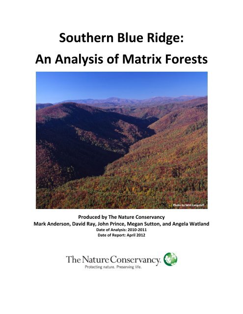
<strong>Southern</strong> <strong>Blue</strong> <strong>Ridge</strong>:<strong>An</strong> <strong>An</strong>alysis <strong>of</strong> <strong>Matrix</strong> <strong>Forests</strong>Photo by Witt LangstaffProduced by The Nature ConservancyMark <strong>An</strong>derson, David Ray, John Prince, Megan Sutton, and <strong>An</strong>gela WatlandDate <strong>of</strong> <strong>An</strong>alysis: 2010-2011Date <strong>of</strong> Report: April 2012
Suggested Citation: <strong>An</strong>derson, M., Prince, J., Ray, D., Sutton, M., and Watland, A. 2013. <strong>Southern</strong> <strong>Blue</strong><strong>Ridge</strong>: an <strong>An</strong>alysis <strong>of</strong> <strong>Matrix</strong> <strong>Forests</strong>. The Nature Conservancy. pp. 51.http://www.conservationgateway.org/Files/Pages/<strong>Southern</strong><strong>Blue</strong><strong>Ridge</strong><strong>An</strong><strong>An</strong>alysis<strong>of</strong><strong>Matrix</strong><strong>Forests</strong>.aspxAcknowledgementsWe would like to thank the Glass Foundation for directly funding the expert meetings that were held inall five states <strong>of</strong> the <strong>Southern</strong> <strong>Blue</strong> <strong>Ridge</strong> and for funding the Forest Block video that was completed(http://www.youtube.com/watch?v=qMvwbaU5RWs).We would like to thank the numerous TNC staff that participated in this analysis including Kristen Austin,Catherine Burns, Deron Davis, Colette DeGarady, Sarah Fraser, Sara Gottlieb, Wade Harrison, MalcolmHodges, Eric Krueger, Merrill Lynch, Katherine Medlock, Sally Palmer, Marek Smith, Rick Studenmund,Randy Tate, Maria Whitehead, and Alex Wyss.We would also like to thank our partners that participated in this process including Jon Ambrose, JoanneBaggs, Rob Baldwin, Allen Boynton, Kevin Caldwell, Ge<strong>of</strong>f Call, Ed Clebsch, Jamey Donaldson, MarshallEllis, Tom Govus, Mark Hall, Steve Hall, Dennis Herman, Stan Hutto, Hugh Irwin, Gary Kauffman,Christine Kelly, Josh Kelly, Nathan Klaus, Tim Lee, Jay Leutze, Jeff Magniez, Joe McGuiness, PatrickMcMillan, Joe Miller, James Padgett, Tom Patrick, Mark Pistrang, Ed Pivorun, Joe Pollard, Mike Schafale,Ed Schwartzman, Vic Shelburn, Curtis Smalling, Tom Waldrop, Jesse Webster, Kendrick Weeks, CarolynWells, Jim Wentworth, Jason Wiesnewski, Lori Williams, Claiborne Woodall, and Pete Wyatt.i
TABLE OF CONTENTSEXECUTIVE SUMMARY .............................................................................................................................1AN APPROACH TO LASTING FOREST CONSERVATION IN THE SOUTHERN APPALACHIANS ..........................................2OVERVIEW: THE SBR MATRIX FOREST BLOCK ANALYSIS PROCESS ......................................................................5DELINEATING MATRIX FOREST BLOCKS ........................................................................................................6SCREENING MATRIX FOREST BLOCKS FOR SIZE AND CONDITION .........................................................................8LAND COVER CRITERIA ..........................................................................................................................................................8SIZE CRITERIA ......................................................................................................................................................................8ELEVATION .......................................................................................................................................................................13GEOLOGY .........................................................................................................................................................................14ECOLOGICAL LAND UNITS ....................................................................................................................................................15EVALUATING AND PRIORITIZING A NETWORK OF MATRIX FOREST BLOCKS ......................................................... 22RESULTS OF ANALYSIS ........................................................................................................................... 23SIZE OF MATRIX FOREST BLOCKS .............................................................................................................. 23CONSERVATION STATUS AND CONDITION OF MATRIX FOREST BLOCKS .............................................................. 24LITERATURE CITED ................................................................................................................................ 29ii
Table 1. Data used to evaluate potential fragmenting features in matrix forest block delineation. ........... 7Table 2. Average Territory Size <strong>of</strong> Characteristic SBR Forest Birds ............................................................. 11Table 3. Ecological Land Units Coding Scheme. .......................................................................................... 16Table 4. Tier 1 <strong>Matrix</strong> Forest Block Size Cohorts and ELU Groups Represented. ....................................... 23Table 5. Tier 2 <strong>Matrix</strong> Forest Block Size Cohorts and ELU Groups Represented. ....................................... 24Figure 1. <strong>Southern</strong> <strong>Blue</strong> <strong>Ridge</strong> Ecoregional Boundaries. ............................................................................... 2Figure 2. Regional Forest <strong>Conservation</strong> Model.. ........................................................................................... 5Figure 3. Minimum Dynamic Area for SBR <strong>Matrix</strong> Forest Blocks. ............................................................... 12Figure 4. <strong>An</strong> example <strong>of</strong> landforms ............................................................................................................. 15Figure 5. <strong>Southern</strong> <strong>Blue</strong> <strong>Ridge</strong> Potential <strong>Matrix</strong> Forest Blocks and Ecological Land Units. ........................ 19Figure 6. <strong>Southern</strong> <strong>Blue</strong> <strong>Ridge</strong> Early <strong>Matrix</strong> Forest Blocks by similar Ecological Land Unit Groupings. ..... 20Figure 7. Prioritized <strong>Southern</strong> <strong>Blue</strong> <strong>Ridge</strong> <strong>Matrix</strong> Forest Blocks. ................................................................ 21Figure 8. SBR <strong>Matrix</strong> Forest Blocks Overlapping GAP Status. ..................................................................... 26Appendix A: State Expert Review Teams and TNC <strong>An</strong>alysis Team Members ............................................. 33Appendix B: Fragmenting Features: Detailed GIS info ............................................................................... 35Appendix C: <strong>Southern</strong> <strong>Blue</strong> <strong>Ridge</strong> Geology Classes..................................................................................... 36Appendix D: <strong>Matrix</strong> Forest Block Information ........................................................................................... 38Appendix E: Final <strong>Southern</strong> <strong>Blue</strong> <strong>Ridge</strong> <strong>Matrix</strong> Forest Block Statistics ....................................................... 41Appendix F: Key to Columns in Appendix E ............................................................................................... 48iii
EXECUTIVE SUMMARYThe <strong>Southern</strong> <strong>Blue</strong> <strong>Ridge</strong> (SBR) Ecoregion’s forested landscape (portions <strong>of</strong> Georgia, North Carolina,South Carolina, Tennessee, and Virginia) is comprised <strong>of</strong> intact temperate forest over a diversity <strong>of</strong>landforms, elevation zones, and bedrock geologies, making it one <strong>of</strong> the most biologically-diverse areasin North America. This region contains several <strong>of</strong> the few remaining mega-blocks <strong>of</strong> relativelyunfragmented forest in the eastern United States, supporting the highest diversity <strong>of</strong> salamanders in theworld, a tremendous diversity <strong>of</strong> tree and herbaceous species, and very high densities <strong>of</strong> forest breedingbirds. These large contiguous forests provide fundamental ecosystem services that sustain underlyingnatural processes, ensuring the continued persistence <strong>of</strong> plant and animal populations as well as theprovisioning, regulating, and cultural ecosystem services on which humans depend (e.g., quality drinkingwater, flood control). From a global perspective, the <strong>Southern</strong> <strong>Blue</strong> <strong>Ridge</strong> forested landscape is a hugeand irreplaceable ecosystem recovering from regional-scale deforestation. These reestablished forestsare facing compounding and interacting threats due to increased human population, forestfragmentation, pests and pathogens, soil acidification and global climate change.Previous efforts by The Nature Conservancy (TNC) and its partners identified priority SBR conservationlocations, focusing largely on occurrences <strong>of</strong> rare species and communities at the scale <strong>of</strong> individualpatches; however, the scope and magnitude <strong>of</strong> today’s conservation challenges mean that we mustexpand our focus to include landscapes and strategies beyond a protected network <strong>of</strong> preserves. TheConservancy’s approach to the long-term conservation <strong>of</strong> the <strong>Southern</strong> <strong>Blue</strong> <strong>Ridge</strong> critical forestresource envisions the conservation <strong>of</strong> a connected, representative, well managed, matrix forests,embedded with large areas <strong>of</strong> core forest(s). The matrix forest blocks sustain natural cover throughmultiple-use working forests, while the core forests are protected and managed for natural ecologicalfunction that promotes biodiversity and natural disturbance regimes (i.e., a dynamic mosaic <strong>of</strong> stands indifferent age and seral classes).This report summarizes the process and results <strong>of</strong> the <strong>Southern</strong> <strong>Blue</strong> <strong>Ridge</strong> <strong>Matrix</strong> Forest <strong>An</strong>alysis,completed in 2011, which identified a representative network <strong>of</strong> matrix forest blocks, large andcontiguous enough to maintain key ecosystem processes and services, resilience, and movement <strong>of</strong>organisms, and to provide for accommodation <strong>of</strong> catastrophic disturbances and the breeding needs <strong>of</strong>forest interior species. In 2011, TNC staff from Eastern North America Division Science and five stateoperating units (with significant contributions from several state and regional partners) completed afour-step analysis process to identify priority SBR matrix forests, involving (1) delineating matrix forestblocks (discrete blocks <strong>of</strong> contiguous forest, using roads and other fragmenting features in GIS), (2)screening each matrix forest block for size and condition using land cover and size criteria, related todisturbance and species’ needs, (3) classifying the matrix forest blocks into representative forestlandscape types, using elevation, geology and landforms (Ecological Land Units), and (4) evaluating andprioritizing a network <strong>of</strong> functional matrix forest blocks representative <strong>of</strong> the diversity <strong>of</strong> ecoregionalforest landscape types, using additional data and expert review.The results give us a much clearer understanding <strong>of</strong> the status, distribution, and spatial context <strong>of</strong> large,contiguous matrix forests in the <strong>Southern</strong> <strong>Blue</strong> <strong>Ridge</strong>, and will provide a clearer direction for near-termconservation priorities and foster a more focused set <strong>of</strong> conservation actions around which TNC andpartners can organize and cooperate. The Nature Conservancy’s vision for the conservation <strong>of</strong> theseidentified priority SBR matrix forest blocks is to work with partners to (1) ensure adequate long-term1
protection and ecologically-compatible management practices, (2) retain connectedness <strong>of</strong> forest coveramong and between them, and 3) work to abate region-wide forest threats.AN APPROACH TO LASTING FOREST CONSERVATION IN THE SOUTHERN APPALACHIANSIf one imagines oneself looking out a plane window on a flight from Atlanta, GA toward Pittsburgh, PA, alarge-scale perspective on the <strong>Southern</strong> <strong>Blue</strong> <strong>Ridge</strong> (SBR) Ecoregion can be visualized (Figure 1). At thiselevation, some <strong>of</strong> the few remaining mega-blocks <strong>of</strong> relatively unfragmented forest in the easternUnited States are readily apparent toeven the untrained eye. For instance,10 <strong>of</strong> the matrix forest blocksidentified in this study are between100,000 and 300,000 acres in size.These forests are important for thepeople inhabiting the region, whodepend on them not only forprovisioning and regulating ecosystemservices (e.g., quality drinking water,natural resource extraction and use,erosion and flood control) but also forcultural services (i.e., the non-materialbenefits and renewal that comes frombeautiful scenery and recreation). Ofcourse, these large contiguous forestsalso provide fundamental ecosystemservices that sustain underlyingnatural processes, ensuring theFigure 1. <strong>Southern</strong> <strong>Blue</strong> <strong>Ridge</strong> Ecoregional Boundaries.continued persistence <strong>of</strong> plant and animal populations as well as the provisioning, regulating, andcultural ecosystem services on which humans depend. The driving force behind these benefits to peopleand the reason the <strong>Southern</strong> <strong>Blue</strong> <strong>Ridge</strong> elicits both scientific and spiritual awe is this ecoregion’s wellrenownedglobally-significant biodiversity (e.g., unique natural communities like globally-rare grassybalds, Carolina hemlock bluffs, and southern Appalachian bogs).The <strong>Southern</strong> <strong>Blue</strong> <strong>Ridge</strong> Ecoregion means many things to many different people. Its 9.4 million acresare home to approximately two million people (US Census 2010), composed <strong>of</strong> some families that havebeen rooted in the land for generations, and others, lured largely by quality-<strong>of</strong>-life factors, that haverecently migrated there. Countless other part-time residents and visitors appreciate the beauty andrecreation <strong>of</strong> the <strong>Southern</strong> <strong>Blue</strong> <strong>Ridge</strong> mountains, valleys, and coldwater streams, including enjoyingscenic vistas along the <strong>Blue</strong> <strong>Ridge</strong> Parkway and within the Great Smoky Mountain National Park, as wellas fishing, hunting, hiking, and biking on 3.2 million acres <strong>of</strong> National Forest. Natural beauty and bountymeet cultural richness in small-to-mid-sized cities like Asheville, NC, Johnson City, TN, and Roanoke, VA,as well as in rural pockets <strong>of</strong> artistic expression like Yancey County, NC, and <strong>Blue</strong> <strong>Ridge</strong>, GA. Theheadwaters <strong>of</strong> the <strong>Southern</strong> <strong>Blue</strong> <strong>Ridge</strong> also influence several large cities, as the sources <strong>of</strong> drinking andrecreational waters for Atlanta, GA, Charlotte, NC, Knoxville, TN, and Greenville, SC. Research showsthat one-third <strong>of</strong> the world’s 105 largest cities’ drinking water sources arise from protected areas,demonstrating the benefit <strong>of</strong> well-managed natural forests to urban populations (Dudley and Stolton2003).2
The <strong>Southern</strong> <strong>Blue</strong> <strong>Ridge</strong> is a forested landscape <strong>of</strong> steeps slopes, high mountains, deep ravines, andwide valleys. The combination <strong>of</strong> intact temperate forest over a diversity <strong>of</strong> landforms, elevation zones,and bedrock geologies, makes it one <strong>of</strong> the most biologically diverse areas in North America. “The regionsupports the highest diversity <strong>of</strong> salamanders in the world, extremely rich forests with a tremendousdiversity <strong>of</strong> tree and herbaceous species, and very high densities <strong>of</strong> breeding birds” (Hunter et al. 1999).Five broad forest types, characteristic <strong>of</strong> the region, form the dominant matrix (Appalachian oakhardwoods, dry oak pine, cove forests, northern hardwoods, andspruce-fir), and their distribution tracks change with elevation. Otherforest types (such as riparian forests) occur at a smaller scale, usually inconjunction with a landform or specific setting. At the scale <strong>of</strong> largeintact forest areas (5,000 – 50,000 acres), the individual forest typesblend and intermix to form a larger functioning unit that shares manyprocesses and exhibits structural and compositional heterogeneity. Eachforest type will display a range <strong>of</strong> successional classes, given the ability<strong>of</strong> various processes and disturbances to play out across the landscape.From a global perspective, the temperate deciduous and mixed forest <strong>of</strong>the <strong>Southern</strong> <strong>Blue</strong> <strong>Ridge</strong> is a huge and irreplaceable ecosystemrecovering from regional-scale deforestation. The great majority <strong>of</strong> thecurrent forest is mid-to-late successional; however much <strong>of</strong> its speciesand structural composition has been altered by past land uses andpractices such as agriculture, pasturing, fire suppression, and logging.Photo by Hugh MortonConcurrent with forest re-establishment, the human population hasincreased exponentially, leading to increased densities <strong>of</strong> roads and other urban environments whichhave led to greater forest fragmentation. Other stresses have expanded to include and compoundhabitat fragmentation, and threats such as increased pests and pathogens, soil acidification and globalclimate change continue to increase.In 2000, The Nature Conservancy (TNC) and its partners (<strong>Southern</strong> Appalachian Forest Coalition andAssociation for Biodiversity Information) conducted an Ecoregional Assessment for the <strong>Southern</strong> <strong>Blue</strong><strong>Ridge</strong>, identifying priority conservation locations (portfolio sites) known to harbor conservation targets(i.e., globally-rare plants, animals, and natural communities) (TNC & SAFC 2000). The EcoregionalAssessment, however, did not include identification and evaluation <strong>of</strong> large contiguous forested habitatsthemselves for conservation priorities, which form the very matrix supporting embedded conservationtargets. The scope and magnitude <strong>of</strong> today’s conservation challenges mean that we can no longerafford to limit our strategies to protecting a network <strong>of</strong> preserves, but must consider strategies andlandscapes large enough to maintain key ecosystem processes and services, resilience, and movement<strong>of</strong> organisms. TNC has recognized the need for this new “whole system” approach that involves workingat multiple scales, with an increasing emphasis on managing for connectivity and a permeable matrix <strong>of</strong>lands and waters that vary in quality, surrounding portfolio sites <strong>of</strong> high ecological integrity. In the<strong>Southern</strong> <strong>Blue</strong> <strong>Ridge</strong>, this means looking across the landscape at large blocks <strong>of</strong> native habitat that cansupport the species, communities, and ecosystem processes and functions that will protect biodiversityand support people’s well-being now and into the future.The first iteration <strong>of</strong> the <strong>Southern</strong> <strong>Blue</strong> <strong>Ridge</strong> Ecoregional Assessment in 2000 (TNC & SAFC 2000)focused largely on rare species and communities or elements <strong>of</strong> biodiversity that occurred at the scale3
<strong>of</strong> individual patches. This follow up study was designed to specifically spatially-define the contiguous,large matrix-forming forest types (herein, “matrix forest”) across the landscape (<strong>An</strong>derson 2008).Developed by TNC operating units in the northern Appalachians, this new assessment for the southernsections <strong>of</strong> the Appalachian Mountains has resulted in a much clearer understanding <strong>of</strong> the status anddistribution <strong>of</strong> matrix forest conservation targets in this ecoregion. This report presents the process,methods, and results <strong>of</strong> the analysis, completed in 2011. It closes a significant gap in our understanding<strong>of</strong> the spatial context and characteristics <strong>of</strong> large contiguous forests in the <strong>Southern</strong> <strong>Blue</strong> <strong>Ridge</strong>, and willprovide a clearer direction for near-term conservation priorities, and foster a more focused set <strong>of</strong>conservation actions around which TNC and partners can organize and cooperate.Scientists have wrestled with how to conserve such a critical but compromised forest resource. TheNature Conservancy’s vision for the conservation <strong>of</strong> this forest includes employing strategies to (1)ensure adequate long-term protection and management <strong>of</strong> a network <strong>of</strong> representative matrix forestblocks, embedded core forests surrounded with working forest buffer (Noss and Cooperrider 1994,Figure 2), (2) retain connectedness <strong>of</strong> forest cover among and between those matrix forests and acrossthe landscape, and 3) abate region-wide forest threats. The identification <strong>of</strong> a representative network<strong>of</strong> matrix forest blocks large enough to sustain forest ecosystem processes is the subject <strong>of</strong> this planningeffort (<strong>An</strong>derson 2008).The Conservancy’s approach to the long-term conservation <strong>of</strong> the <strong>Southern</strong> <strong>Blue</strong> <strong>Ridge</strong> critical forestresource envisions the conservation <strong>of</strong> a connected, representative, well managed, matrix <strong>of</strong> forest,embedded with large core forest areas. The matrix sustains natural cover through multiple-use workingforests, while the core forests are protected and managed for natural ecological function that promotesbiodiversity and natural disturbance regimes. The desired condition <strong>of</strong> embedded core forest is not asolid stand <strong>of</strong> old-growth trees, but rather, a mosaic <strong>of</strong> stands in different age classes, from early to latesuccessional, that retain biological legacies (such as coarse woody debris and standing snags), andreflect the natural disturbance regimes <strong>of</strong> the region. This assessment describes the delineation <strong>of</strong>matrix forest areas large enough to provide for accommodation <strong>of</strong> catastrophic disturbances and thebreeding needs <strong>of</strong> forest interior species. Our methods anticipate forest matrix blocks that include arange <strong>of</strong> habitats and a shifting mosaic <strong>of</strong> seral stages (see section on Size in Relation to Disturbances).4
Figure 2. Regional Forest <strong>Conservation</strong> Model (adapted from Noss and Cooperridge 1994). Thisdisplays the concept <strong>of</strong> a model regional reserve network, consisting <strong>of</strong> core forests, connectingcorridors or linkages, and multiple-use buffer zones. “<strong>Matrix</strong> forests” refer to the overall contiguousforested landscape, while “core forests” refer to areas managed for natural ecological integrity.Inner buffer zones would be strictly protected, while outer buffer zones would allow for a widerrange <strong>of</strong> compatible human uses. The inter-regional corridor connects this system to a similarnetwork nearby.OVERVIEW: THE SBR MATRIX FOREST BLOCK ANALYSIS PROCESSThe <strong>Southern</strong> <strong>Blue</strong> <strong>Ridge</strong> <strong>Matrix</strong> Forest Block <strong>An</strong>alysis was a joint effort among TNC’s Eastern NorthAmerica Division Science staff and staff from the five TNC state operating units partially within theecoregion (Georgia, North Carolina, South Carolina, Tennessee, and Virginia). Significant contributionsand feedback were also provided by several state and regionalpartners (Appendix A). This process was similar to theConservancy’s matrix forest analysis in the CentralAppalachian and Northern Appalachian Ecoregions t<strong>of</strong>acilitate regional consistency in the identification andevaluation <strong>of</strong> Appalachian spatial conservation targets andecological goals. The major steps and details <strong>of</strong> the analysisprocess are summarized in this report, and supportingdocuments and additional details can be found at:http://www.conservationgateway.org/Files/Pages/<strong>Southern</strong><strong>Blue</strong><strong>Ridge</strong><strong>An</strong><strong>An</strong>alysis<strong>of</strong><strong>Matrix</strong><strong>Forests</strong>.aspx.5
We developed a four-step analysis process to assess, prioritize, and direct conservation strategies toprotect the <strong>Southern</strong> <strong>Blue</strong> <strong>Ridge</strong> matrix forest system:• Delineate matrix forest blocks to identify and subdivide the forested landscape into discrete blocks<strong>of</strong> contiguous forest, using roads and other fragmenting features in GIS.• Screen each matrix forest block for size and condition using land cover and size criteria, related todisturbance and species’ needs.• Classify the candidate matrix forest blocks into multiple groups that reflect similar combinations <strong>of</strong>elevation, geology, and landforms (Ecological Land Units).• Evaluate and prioritize a network <strong>of</strong> functional matrix forest blocks representative <strong>of</strong> the diversity<strong>of</strong> ecoregional forest landscape types, using additional data and expert review.DELINEATING MATRIX FOREST BLOCKSUsing GIS data, we subdivided the entire forested landscape <strong>of</strong> the <strong>Southern</strong> <strong>Blue</strong> <strong>Ridge</strong> into discreteunits (“matrix forest blocks”), bounded on all sides by major roads (road classes 1-4; ESRI 2009), lakes,or large rivers (>3,681m 2 drainage area) (USEPA and USGS 2008) (Table 1 and Appendix B). Roads werean appropriate choice for this task, as they disrupt the movement <strong>of</strong> some organisms and the flow <strong>of</strong>some ecological processes, and they increase the level <strong>of</strong> access into interior forest areas. Additionally,we analyzed and sometimes adjusted blocks according to the location <strong>of</strong> roads, railroads, powerlines,logging trails, housing developments, agricultural lands, and mining operations from obtained digitaldata or aerial imagery (Table 1) that can be highly correlated with human natural resource extractive orother ecologically-incompatible activities that can impair connectivity and forest processes. DelineatedSBR matrix forest blocks were bounded on all sides by connected fragmenting roads (or other features),forming polygons that completely encircled large contiguous patches <strong>of</strong> forest. However, delineatedblocks are not necessarily roadless, as blocks can contain intersecting roads (roads that extend intoblock boundaries, but do not bisect the block).6
Table 1. Data used to evaluate potential fragmenting features in matrix forest block delineation.PotentialFragmentingFeatureRoadsData <strong>An</strong>alyzed(Year)Streetscarto layerfrom ESRI GIS data(ESRI 2009)Description <strong>of</strong> <strong>An</strong>alysisDetailed road data was evaluatedagainst aerial imagery (accessedusing Google Earth and ArcGISOnline 2010-2011) to determineaccuracy and completeness <strong>of</strong> roadcoverage.Final Decision: FragmentingFeature?Road classes 1 through 4, which roughlyequates to Interstates (1), U.S. Routes andsome State Routes (2), State Routes and oldhighways (3), and exit and on ramps, serviceroads, and rest area roads (4), weredetermined to be fragmenters.PowerlinesRailroadsVentyx powerlinetransmission data(Ventyx 2010)Ventyx Railroaddata (Ventyx 2010)Powerline Transmission data wasevaluated against aerial imagery(accessed using Google Earth andArcGIS Online 2010-2011) to assessvegetation cuts (width andmanagement intensity).Railroad corridors were evaluatedagainst aerial imagery (accessedusing Google Earth and ArcGISOnline 2010-2011) to assessvegetation gaps (width,management, tunnel openings, andadjacency to roads/ rivers).Due to high variability <strong>of</strong> the width <strong>of</strong> thepowerlines and the degree to which theywere maintained as cut areas across theregion, powerlines were not uniformlyviewed as fragmenting features but wereconsidered on a case-by-case basis; wherepowerlines were large in width and requiredvegetation management continuouslythroughout individual blocks, these wereviewed as fragmenters.Due to sporadic traffic and <strong>of</strong>ten narrowopenings made for trains, railroads were notviewed as uniform fragmenting features;railroad attributes (width, management,tunnel openings, and adjacency toroads/rivers) were considered as potentialfragmenters within individual blocks.LakesNationalHydrographyDatabase (USEPAand USGS 2008)Waterbodies were evaluated todetermine if they created significantgaps in forest canopy.Determined to be fragmenting features.RiversNationalHydrographyDatabase (USEPAand USGS 2008)Waterbodies were evaluated todetermine if they created significantgaps in forest canopy.Large rivers or stream segments (draining>3,861 miles 2 ) were determined to befragmenting features.Developed/DisturbedAreasSE GAP NLCD 2006land cover (Fry etal. 2011)Land cover data was utilized tovisually assess fragmentation <strong>of</strong>forest cover.Not used as fragmenting features duringinitial block identification. Somemodifications to blocks were manually madebased on this later in the process.7
SCREENING MATRIX FOREST BLOCKS FOR SIZE AND CONDITIONOur work to identify a network <strong>of</strong> representative forest reserves posed several important questionsrelated to the size and condition <strong>of</strong> matrix forest blocks: How large must a forest reserve be to remainresilient in the face <strong>of</strong> a changing climate? How large must it be to contain all <strong>of</strong> its expectedbiodiversity? How can we tell if a forest occurrence has integrity with regard to its internal processes?In this section, we describe the criteria developed to identify qualifying matrix forest blocks in thisanalysis.Our goal was to identity matrix forest blocks large enough to function as viable, resilient forestecosystems. At a minimum, we assumed that a viable matrix forest patch includes both the biota andthe functions that arise from their interactions (e.g. pollination, decomposition), and the intactness <strong>of</strong>the physical setting and external processes that sustain the ecosystem (Forman 1995, Franklin 1993).Further, our working definition <strong>of</strong> resilience was the ecosystem’s “capacity to renew itself or adaptwithin a dynamic environment” (Gunderson 2000). We assumed that viable, resilient systems are morelikely to persist, not in a static manner but in a dynamic state that fluctuates within some bounds <strong>of</strong>variation or that adjusts gradually to new situations if the underlying environmental conditions change.Under a changing climate, the individual species that compose the system may change in abundance,and new species may be introduced to the system, but overall the forest continues to support a diversity<strong>of</strong> species and maintain its essential processes.LAND COVER CRITERIATo ensure that this analysis focused on the identification <strong>of</strong> contiguous forest, we used the SE GAP landcover GIS database (2008) to tabulate the amount <strong>of</strong> forest cover within each potential matrix forestblock. All blocks containing at least 80% forest cover qualified for further review.SIZE CRITERIAThe ability <strong>of</strong> a forest patch to provide adequate breeding territories for multiple pairs <strong>of</strong> forest interiorspecies, and to remain resilient under a suite <strong>of</strong> expected large disturbances, is correlated with its size(Poiani et al 2000, <strong>An</strong>derson 2008). To understand the matrix forest block size necessary for effectiveforest conservation in this region, we identified two independent sets <strong>of</strong> size criteria, using (a) the scaleand frequency <strong>of</strong> natural disturbances to estimate the minimum dynamic area, and (b) the breedingarea requirements <strong>of</strong> interior-forest specialist bird species, to ensure that conserved matrix forests are<strong>of</strong> adequate size to function as a “coarse-filter” habitat for associated species, accommodating a broadrange <strong>of</strong> seral stages, at different elevations (Hunter 1996).Size in Relation to DisturbanceTo persist over time, a forest block must be large enough to absorb large, infrequent, disturbances.Natural disturbances, although catastrophic relative to the mortality <strong>of</strong> living trees, ultimatelyrejuvenate ecosystems by releasing and redistributing resources, and creating successional habitat thatfavors a different set <strong>of</strong> species. Spatial variation in disturbance severity and frequency breakshomogeneous areas into a mosaic <strong>of</strong> overlapping heterogeneous patches, and keeps the system in adynamic state <strong>of</strong> flux. The area necessary to maintain processes and ensure persistence has been calledthe system’s minimum dynamic area (Pickett and Thompson 1978).Primary natural disturbances in the <strong>Southern</strong> <strong>Blue</strong> <strong>Ridge</strong> are fire, drought, floods, tornadoes, hurricanes,ice storms, landslides, pathogens, and insects. Some sites, because <strong>of</strong> their position along environmental8
gradients, are more prone to certain disturbances. For example, ice damage occurs more frequently atcooler and higher elevations, wind-throw is more likely on exposed slopes, drought mortality is morefrequent on ridge sites, and fires are more likely on dry, warm, low-elevation southern exposures.To estimate the minimum dynamic area needed to absorb the largest likely disturbance over the course<strong>of</strong> several centuries, we collected and reviewed published information and expert knowledge on thelargest known disturbance patch sizes created by wind and fire in the SBR. We multiplied thesedisturbance patch sizes by four, theorizing that resilience would be enhanced if less than one-quarter <strong>of</strong>the forest block was in the immediate stages <strong>of</strong> recovery at any one time (<strong>An</strong>derson 2008). Weemphasize that this is a ballpark estimate, as there is much more detailed research underway to identifyoccurrence probabilities for forest patch sizes <strong>of</strong> varying disturbances. Ideally, one would model variousdisturbances in specific areas to extract the maxima and minima and other distributional information (D.L<strong>of</strong>tis pers. com.). By scaling to the four-times the largest recorded damage patch, we attempt toidentify a robust size criterion to allow for a variety <strong>of</strong> scenarios to play out.In the <strong>Southern</strong> <strong>Blue</strong> <strong>Ridge</strong>, wind disturbance (tornadoes, hurricanes, and downbursts) primarily createssmall gaps on the scale <strong>of</strong> 0.1 acre (5-6 m 2 ) and ranging up to 2.7 acres (0.2-1.1 ha). New gaps form at anaverage rate <strong>of</strong> 1% <strong>of</strong> total land area per year, and in sample areas covered 9.5% <strong>of</strong> the land area(Runkle 1981, Runkle 1982, Greenberg and McNab 1998, Ventyx 2010). A recent tornado touched downin the western tip <strong>of</strong> the Great Smoky National Park in April <strong>of</strong> 2011, creating a disturbance patch 11.5miles long and one-quarter mile wide, equivalent to 2,080 acres in size (D. Ray, pers. comm.). Using thisinformation, the estimated minimum dynamic area (four-times largest known disturbance size) wouldbe 0.4 acres for small wind disturbance gaps, 10.8 acres for hurricane downbursts, and 8,320 acres fortornado damage patches in the <strong>Southern</strong> <strong>Blue</strong> <strong>Ridge</strong>.The role <strong>of</strong> fire in the <strong>Southern</strong> <strong>Blue</strong> <strong>Ridge</strong> is not well understood, but it is likely that the fire regimes <strong>of</strong>the mountains are distinct from the well-studied Piedmont and Coastal Plain. There is evidence that fireshave regularly burned across some mountainous areas over the past 4,000 years, although theseasonality and severity <strong>of</strong> these fires remains unknown (Fesenmyer and Christensen 2010). Recentstudies in the nearby Central Appalachians found the average disturbance size <strong>of</strong> 344 natural burns was3 acres (1.2 ha) and the largest known natural fire was 2,938 acres (1,189 ha, Lafon et al 2005). In astudy on Tennessee and North Carolina forest fires, the average disturbance size <strong>of</strong> 126 lighting-causedfires was 2 acres (8 ha), with the largest lightning fire on record burning 81 acres (33ha) (Barden andWoods 2008). Evidence suggests that fires throughout the <strong>Southern</strong> <strong>Blue</strong> <strong>Ridge</strong> similarly occur, mainly aslow intensity burns. Scaling up to four-times the largest known natural fire damage area, the estimatedminimum dynamic area would be 11,752 acres for fire disturbances.Size in Relation to SpeciesTo understand the area needs <strong>of</strong> species associated with <strong>Southern</strong> <strong>Blue</strong> <strong>Ridge</strong> forests and forest interiorhabitat, we identified a set <strong>of</strong> species typical <strong>of</strong>, or restricted to, this ecoregion and used availableinformation on home range, resource, or breeding habitat needs to determine the minimum forest sizearea requirements. We restricted the analysis to vertebrates, as they are usually the most spacedemandingand wide-ranging, and therefore assumed that the space requirements <strong>of</strong> smaller specieswould be met at sizes sufficient for representative vertebrates. We focused on bird species requiring orassociated with forest interior habitat, as these species have the most restrictive requirements withregard to forest size (Martin and Finch 1995). The effects <strong>of</strong> forest patch size and forest fragmentationon particular species (specifically on migratory songbirds) have received extensive attention in the9
literature, and it is well documented that the density <strong>of</strong> many neotropical forest dwelling bird species isgreater in large forested tracts than small forested tracts (Robbins et al. 1989, McIntyre 1995). Thedifferences may be due to: increased pairing success, more suitable foraging or nesting sites, decreasedcompetition for resources, decreased nest predation and/or decreased nest parasitism (Paton 1994,Hartley and Hunter 1997, Fahrig 2003).The <strong>Southern</strong> <strong>Blue</strong> <strong>Ridge</strong> ecoregion supports an estimated 155 species <strong>of</strong> breeding birds (Hunter et al.1999). Nearly 62% <strong>of</strong> all these species are associated with forest habitats, ranging in size from smallwoodlots and groves at lower elevations, to large, extensively forested tracts at mid to high elevations.Low elevation forests support six species <strong>of</strong> woodpeckers, along with many songbird species. Forestpatches at higher elevations contain species that use mid-to-late- successional spruce-fir forests asbreeding or foraging habitat (Hamel 1992). Hunter et al. (1999) estimated that 49 species <strong>of</strong> neotropicalmigrant birds are forest-dependent, and 14 species are associated with wetland or riparian habitats.Population declines have been evident since 1996 in nearly 70% <strong>of</strong> nearctic-neotropical migrant birdspecies that breed in mid-to-late successional forests, while 26% have declined significantly. In addition,31% <strong>of</strong> wetland and riparian neotropical migrants have also declined (Hunter et al. 1999), andpopulations <strong>of</strong> most disturbance-dependent bird species (e.g., golden-winged warbler) in eastern NorthAmerica have declined steeply (Hunter et al. 2001).Breeding territory sizes, home ranges, and resource needs for characteristic forest-interior specialist birdspecies were compiled from Birds <strong>of</strong> North America (Poole and Gill 1992-ongoing). To determine the sizeneeded for matrix forest block occurrences to contain multiple populations and potentially function as asource area for breeding species, we multiplied the average female territory size by 25, using theguideline that at least 50 genetically-effective individuals are necessary to conserve genetic diversitywithin a metapopulation over several generations (Lande 1988). In using this guideline, we wereapproximating the area needed to accommodate 25 breeding females within a single patch <strong>of</strong> forest,not the needed population size to sustain the species, which would be much larger. Results show thatthe territory sizes <strong>of</strong> SBR forest interior bird specialists ranged from 2 acres to over 1000 acresdepending on the species (Table 2).10
Table 2. Average Territory Size <strong>of</strong> Characteristic SBR Forest Birds(compiled by M. Lynch and supplemented by Poole et al. 2012).Average<strong>Southern</strong> <strong>Blue</strong> <strong>Ridge</strong> Birds 1 Territory(Acres)Acres X 25Early SuccessionalGolden-winged Warbler 2 50Vesper Sparrow 10.4 260Cove HardwoodsAcadian Flycatcher 2.7 68Black-throated <strong>Blue</strong> Warbler 2 50Cerulean Warbler 2.6 65Louisiana Waterthrush 1.3 33Swainson's Warbler 2 50Hemlock-White Pine-Mixed HardwoodsBlackburnian Warbler 3 75Black-throated Green Warbler 1.5 38High Elevation HardwoodsRuffed Grouse 5.4 135Yellow-bellied Sapsucker 14 350Black-billed Cuckoo 15 375<strong>Blue</strong>-headed Vireo 0.7 18Rose-breasted Grosbeak 2.5 63Veery 0.5 13Spruce-FirBlack-capped Chickadee 10 250Brown Creeper 11 275Northern Saw-whet Owl 247 6175Red-breasted Nuthatch 12.6 315Golden-crowned Kinglet 2 50Winter Wren 7.2 180Large TerritoryBarred Owl 600 15,000Common Raven 1,200 30,000Cooper's Hawk 500 12,500Broad-winged Hawk 569 14,224To determine the matrix forest block size necessary for effective forest conservation in this region, weplotted these SBR forest-interior species’ area requirements on the same scale as the collecteddisturbance patch minimum dynamic area estimates (Figure 3). For instance, a 1,000 acre patch <strong>of</strong> forestprovides adequate space for 25 breeding pairs <strong>of</strong> yellow-bellied sapsuckers and red breasted warblers,1 Additional requirements beyond size exist for breeding success for many birds, especially early successionalspecies.11
ut is below the size needed for northern saw-whet owls, and is less than half the size <strong>of</strong> the largestsevere fire recorded in the area.In reviewing these results, it was evident that a 15,000 acre forest would be adequate for all the speciesand disturbances examined. We therefore decided to use 15,000 acres <strong>of</strong> contiguous forest as our basesize criteria, but to still evaluate blocks in the smaller size range <strong>of</strong> 10,000-15,000 acres, because weexpected that large blocks may not be available in certain environments (rich soils for example) and the10,000 acre block size would still be adequate for most disturbances and species (in the end all the Tier1 blocks were greater than 15,000 acres in size but some <strong>of</strong> the Tier 2 blocks and connectors weresmaller). Thus our minimum size criterion for viable SBR matrix forest blocks was 15,000 acres. This sizewill provide adequate breeding territories for multiple pairs <strong>of</strong> forest interior species, and can remainresilient under a suite <strong>of</strong> expected severe wind and fire disturbances <strong>of</strong> all types.Figure 3. Minimum Dynamic Area for SBR <strong>Matrix</strong> Forest Blocks, known disturbance patch sizesand select interior-forest breeding specialists’ territory sizes. The blue circle indicatesapproximately where the 15,000 acre criteria stand in relation to the other features.12
CLASSIFYING THE MATRIX FOREST BLOCKS<strong>An</strong> understanding <strong>of</strong> patterns <strong>of</strong> environmental variation and biological diversity is fundamental toconservation planning at any scale—regional, landscape level, or local. Moreover, maintaining forestbiodiversity through a forest reserve network is a trade<strong>of</strong>f between distributing risk over many reservesrepresenting the full spectrum <strong>of</strong> environmental settings (the goal <strong>of</strong> this analysis stage) and minimizingthe probability <strong>of</strong> loss in each individual reserve (the goal <strong>of</strong> the size criteria analysis stage).In order to identify a representative network <strong>of</strong> matrix forest blocks, a dataset was developed to assessthe geophysical character <strong>of</strong> the landscape, which can also be used to approximate the distribution andcomposition <strong>of</strong> many community assemblages across those landscapes. The close relationship <strong>of</strong> thephysical environment to ecological process and biotic distributions underpins the ecological sciences,and given the changing climate and associated changing species distributions, geophysical diversity maybe an appropriate target for conservation planning (<strong>An</strong>derson and Ferree 2010) Research has repeatedlydemonstrated especially strong links between ecosystem pattern and processes, climate, bedrock, soils,and topography.To quantify the physical diversity <strong>of</strong> the <strong>Southern</strong> <strong>Blue</strong> <strong>Ridge</strong>, we developed individual 30m cell GISdatasets <strong>of</strong> elevation, geology, and landforms, and integrated them into a single unit called theEcological Land Unit (ELU). Each ELU code represents a specific landform (e.g., cove), composed <strong>of</strong> aspecific bedrock type (e.g., calcareous), within a specific elevation zone (e.g., low elevation). The ELUdataset describes only the physical information, but it can be combined with land use or land covermaps to approximate vegetation types. We present a brief description <strong>of</strong> each <strong>of</strong> the ELU dataset layersbelow.ELEVATIONElevation is a strong predictor <strong>of</strong> the distribution <strong>of</strong> forest communities. Temperature, precipitation,and exposure commonly vary with changing altitude, as does the dominant vegetation type. Red sprucebegins to occur within northern hardwood forests at around 1,405m (4,500ft) and becomes moredominant with increasing elevation. Fraser fir species abundance increases above 1,720m (5,500ft) andcan occur in pure stands over 1,875m (6,000ft). Hemlock-dominated forests, along with white pine andhardwood mixed habitats, occur at middle elevations and <strong>of</strong>ten in small stands along north-facing slopesat elevations between about 762-1,220m (2,500-4,000ft). Variations <strong>of</strong> cove forest can be foundthroughout the <strong>Southern</strong> Appalachians at elevations from 305 to 1,372m (1,000-4,500ft). Appalachianoak forests composed <strong>of</strong> northern red, chestnut, white, and black oaks, in combination with many otherspecies (especially pignut and mockernut hickory and red maple) typically occur at elevations from 250mto 1,280m (820-4,200ft) elevations (Stephenson et al. 1993, Hunter et al. 1999).We used the following elevation cut<strong>of</strong>fs to map distinct elevation zones:Very HighHighMedium HighMedium LowLow5,500ft+4,200-5,500ft3,500-4,200ft2,300-3,500ft2,300ft or less13
GEOLOGYBedrock geology strongly influences area soil and water chemistry. Bedrock types also differ in howthey weather and in the physical characteristics <strong>of</strong> the residual soil type. Because <strong>of</strong> this, local lithologyis usually the principle determinant <strong>of</strong> soil chemistry, texture, and nutrient availability. Many ecologicalcommunity types are closely related to the chemistry and drainage <strong>of</strong> the soil or are associated withparticular bedrock exposures.We grouped bedrock units on the bedrock geology maps <strong>of</strong> Virginia, North Carolina, Tennessee, SouthCarolina, and Georgia into nine general classes, designed to have particular relevance to vegetationdistributions. The nine categories listed below were based on the chemical and physical properties <strong>of</strong>the soils derived from them, and are correlated with regional biodiversity patterns (<strong>An</strong>derson and Ferree2010, Appendix C).Acidic sedimentary: Fine to coarse-grained, acidic sedimentary or meta-sedimentary rock. This groupincludes: mudstone, claystone, siltstone, non-fissile shale, sandstone, conglomerate, breccia, greywacke,and arenites. Metamorphic equivalents inlcude: slates, phyllites, pelites, schists, pelitic schists, andgran<strong>of</strong>els.Acidic shale: This group includes any fine-grained loosely compacted acidic fissile shale.Calcareous: Alkaline, s<strong>of</strong>t, sedimentary or metasedimentary rock with high calcium content. This groupincludes: limestone, dolomite, dolostone, marble, and other carbonate-rich clastic rocks.Moderately Calcareous: Neutral to alkaline, moderately s<strong>of</strong>t sedimentary or meta-sedimentary rockwith some calcium but less so than the calcareous rocks. This group includes: calcareous shales, pelitesand siltstones, calcareous sandstones, lightly metamorphosed calcareous pelites, quartzites, schists andphyllites, and calc-silicate gran<strong>of</strong>els.Acidic Granitic: Quartz-rich, resistant acidic igneous and high grade meta-sedimentary rock. This groupincludes: granite, granodiorite, rhyolite, felsite, pegmatite, granitic gneiss, charnockites, migmatites,quartzose gneiss, quartzite, and quartz gran<strong>of</strong>el.Mafic: Quartz-poor alkaline to slightly acidic rock. This group includes: (ultrabasic) anorthosite (basic),gabbro, diabase, basalt (intermediate), quartz-poor: diorite/ andesite, syenite/ trachyte, greenstone,amphibolite, epidiorite, granulite, bostonite, and essexite.Ultramafic: Magnesium-rich alkaline rock. This group includes: serpentine, soapstone, pyroxenites,dunites, peridotites, and talc schist.Coarse Surficial Sediment: This group includes deep unconsolidated sand and gravel.Fine Surficial Sediment: This group includes deep unconsolidated silt and mud.14
LANDFORMLandforms anchor and control terrestrial ecosystems by breaking broad landscapes into localtopographic units and creating meso- and micro-climates. Topography is largely responsible for localvariation in solar radiation, soil development, moisture availability, and susceptibility to wind and otherdisturbances. To map SBR ecoregional landforms, we created an 11-part GIS landform model thatdelineated local environments, representing distinct combinations <strong>of</strong> moisture, radiant energy,deposition, and erosion. The model, based on land surface models developed for soil mapping,categorizes various combinations <strong>of</strong> slope, land position, aspect, and moisture accumulation.Development methods were based on Fels and Matson (1997) and are described in detail in <strong>An</strong>derson etal. 2012. The model is derived from a 30-meter Digital Elevation Model and maps the followinglandforms (Figure 4):1) Cliff or steep slope (includes cliffs and steep slopes <strong>of</strong> warm and cool aspects)2) Summit or ridgetop (includes flat summit, upper ridges, and slope crests)3) Northeast sideslope (includes moderately steep sideslopes <strong>of</strong> cooler aspects)4) Southwest sideslope (includes moderately steep sideslopes <strong>of</strong> warmer aspects)5) Cove or slope bottom (includes slope bottom flats, and coves <strong>of</strong> warm and cool aspects)6) Low hill7) Low hilltop flat8) Valley or toeslope9) Dry flat10) Wet flat11) Water (includes lakes, ponds,rivers and estuaries)ECOLOGICAL LAND UNITSTo integrate the elevation, geology, andlandform characteristics, we used GIS tocode every 30-meter cell in the regionwith its elevation zone, geology class,and landform type. For example, a cell at1,400 feet (elevation class 2000) ongranitic bedrock (substrate class 500) in awet flat (landform 31) would be coded2531 (Figure 4, Table 3). In total, the<strong>Southern</strong> <strong>Blue</strong> <strong>Ridge</strong> Ecoregion had 453unique combinations <strong>of</strong> elevation zone,substrate type, and landform. TheseELU data were used to provide anabiotic characterization <strong>of</strong> each <strong>of</strong> thecandidate matrix forest blocks (Figure5).Figure 4. <strong>An</strong> example <strong>of</strong> landforms, used for Ecological Land Unitdevelopment, in Linville Gorge Wilderness Area in North Carolina.15
Table 3. Ecological Land Units Coding Scheme.Elevation class (ft) + Substrate class + Landform1000 (0-2300) 100 acidic sed/metased 4 steep slope2000 (2300-3500) 200 acidic shale 5 cliff3000 (3500-4200) 300 calc sed/metased 11 flat summit/ridgetop4000 (4200-5500) 400 mod. calc sed/metased 13 slope crest5000 (> 5500) 500 acidic granitic 21 Hilltop (flat)600 mafic/intermed granitic 22 Hill (gentle slope)700 ultramafic 23 NW-facing sideslope800 coarse sediments 24 SE-facing sideslope900 fine sediments 30 Dry flat31 Wet flat32 Valley/toe slope41 Flat at bottom <strong>of</strong> steep slope43 NW-facing cove/draw44 SE-facing cove/draw51 Polygonal rivers from NHD52 NHD lakes/ponds/reservoirsClassifying <strong>Matrix</strong> Forest Blocks by ELU ComponentsWe overlaid potential matrix forest block boundaries (meeting size and land cover criteria as describedabove) with the ELU data layer, and tabulated the area <strong>of</strong> each unique ELU code within each block,summarizing the types and amounts <strong>of</strong> physical features contained. We used this information to classifythe forest blocks, using a standard quantitative cluster analysis (CLUSTER and TWINSPAN) within PC-ORDversion 6 (McCune and Mefford 1992, McCune and Grace 2002) to aggregate the forest matrix blocksinto groups that shared a similar combination <strong>of</strong> physical features. This ordination process resulted ingroups <strong>of</strong> similar recognizable forest-landscape combinations, which we termed “ELU groups” (Figure 6).16
The analysis resulted in 25 ELU groups, based largely on differences in elevation zones and geologytypes. Among ELU groups, the types and proportions <strong>of</strong> landforms varied less (the largest variationswere related to the proportion <strong>of</strong> flats and wet flats in each block). We further subdivided some <strong>of</strong> thegroups into subgroups (labeled a, b, or c) based on both ecological characteristics and the geographicdistribution <strong>of</strong> the blocks. For example if a group contained two spatially-disjunct sets <strong>of</strong> blocks thatwere found in different physiographic regions, we split that ELU group into subgroups (Figure 6).The resulting ELU groups and subgroups, and the names <strong>of</strong> the matrix forest blocks they contain, arelisted below (arranged by elevation zone):LOW ELEVATION• Group 3: Low elevation acidic sedimentary blocks, mostly sideslopes with coves prevalent –Examples: Fort Mt., Hiwassee, Hiwassee Lake, Web Mt.• Group 4: Low elevation, mix <strong>of</strong> granite and acidic sedimentary, no summits, mostlysideslopes - Examples: Lower Chattooga, Mid-Chattooga, Sumter• Group 13b: Low elevation block on granite and mafic bedrock, steep landforms, valleys fewflats - Examples: South Mt. ConnectorLOW to MID ELEVATION• Group 1: Low to mid elevation, mixed acidic sedimentary and shale, mostly slopes -Examples: Cohutta, Lover's Leap, Sol Messer Mt., Meadow Creek Mt., Starr Mountain• Group 2: Low to mid elevation, acidic sedimentary with bits <strong>of</strong> granite or mafic, mostlysideslope - Examples: Amicalola West, Burnt/Sassafras, Dahlonega/Amicalola, Payne Mt.• Group 5: Low to mid elevation with acidic sedimentary, granite and mafic bedrock. Slopes,few flats - Examples: Bull Mountain, Fairy Stone, Pinnacles <strong>of</strong> Dan• Group 8: Low to mid elevation, very diverse geo: acidic sedimentary, granite, moderatelycalcareous and calcareous. Mostly steep features, few gentle hills - Examples: Max Patch• Group 13a: Low to mid elevation on moderately calcareous and granite bedrock, various landforms - Examples: Adams Mt., Globe, Linville Gorge• Group 14a: Low to mid elevation on granite and coarse surficial sediment. Sideslope, no wetflats - Examples: Poor Mountain• Group 14b Mid to low elevation on granite, Mostly slopes and slope crests, no wet flats -Examples: Mack’s Mountain• Group 14b Mid to low elevation on granite, Mostly slopes and slope crests, no wet flatsExamples: Mack’s Mountain• Group 14c: Mid to low elevation on granite, variety <strong>of</strong> landforms no wet flats Examples:Horse Trough Mt., Raven Cliffs, Unicoi, Blood Mt.• Group 15: Low to mid elevation on granite or with bits <strong>of</strong> mafic and mod calc, variouslandforms Examples: Honeycut Mt./Humpback Mt., Little Switzerland, Doughton/Stone Mt., Elk<strong>Ridge</strong>, Rendezvous Mt., Vannoy, Yadkin Headwaters, Bent Mountain• Group 16-18: Low to mid elevation on granite with substantial component <strong>of</strong> acidicsedimentary, sideslopes and a wide variety <strong>of</strong> landforms Examples: <strong>Blue</strong> Wall, Green River,Chimney Rock, Great Smokies West, Hickory Nut Gorge, Jocassee, Mt. Bridge, Mt. Bridge West,Spring Creek Mt., Headwaters, Tiger, Upper Chattooga/Whitewater, Duncan <strong>Ridge</strong>, Rocky Mt.,Asheville Watershed, Grandfather Mt.17
MID ELEVATION• Group 6: Mid elevation block <strong>of</strong> calcareous limestone with steep slopes and sideslopes -Examples: Doe Mt.• Group 22-24: Mid elevation blocks on granite, coves prevalent along with sideslope, steepslopes - Examples: Big Bald, Roan Mt West, Cowee, Cullasaja, Newfound Mountains,Panthertown Valley, Pink Beds, Standing Indian, Looking Glass, Mt. Pisgah, Roy Taylor, RichlandBalsam, Shining Rock• Group 25: Mid elevation blocks with substantial mafic bedrock. Mostly sideslope - Examples:Amphibolite Mts., Roan Mt. East• Group 19b: Mid elevation block on granite, sideslopes and steep slope - Examples: Cathy'sCreek, N. Fork French Broad, Mount Rogers• Group 19a: Mid elevation on granite with substantial acidic sedimentary. Mostly sideslopeand valley - Examples: Dupont, Dupont West• Group 20b: Mostly mid- elevation and mostly granite and a variety <strong>of</strong> landforms - Examples:Big Laurel, Hurricane Mts., Pond Mt., Unaka , Mt. WilderMID to HIGH ELEVATION• Group 10: Mid to high elevation with moderately calcareous and acidic sedimentary. Mostlyslopes - Examples: Nantahala• Group 21: Mid to high elevation with limestone and granite, mostly sideslopes, and steepslopes - Examples: Jefferson/Iron Mt., Sugar GroveALL ELEVATION ZONES• Group 7: Diverse blocks with many elevation zones, and many types <strong>of</strong> sedimentarybedrocks. No wet flats, mostly sideslopes and steep slopes - Examples: Buffalo Mountain,Holsten Mt., Rocky Fork, Scioto-Stone Mt. Stone Mountain, The Snake• Group 9: All elevation zones, sedimentary bedrock with sideslopes, steep slopes and coves -Examples: Brasstown Bald, Cheoah, Cove Mt. WMA, Fires Creek, Great Smokies East, HarmonDen, Joyce Kilmer/Unicoi, Rich Mt., Yellow Creek• Group 11: All elevation zones on sedimentary and granite. Mostly sideslopes and steepslopes - Examples: Black Mts., Little Tennessee, Plott Balsams, Qualla, Rabun Bald• Group 12: All elevation zones, diverse blocks with granite, sedimentary and shale no flats orgentle slopes <strong>of</strong> any kind - Examples: Forge Mt. /Mt. Rogers, Nolichucky• Group 20a: All elevation zones and equal parts granite and sedimentary. Steep slopes, withfew flats or gentle slopes - Examples: Chunky Gal, Tri-County18
Figure 5. <strong>Southern</strong> <strong>Blue</strong> <strong>Ridge</strong> Potential <strong>Matrix</strong> Forest Blocks and Ecological Land Units.19
Figure 6. <strong>Southern</strong> <strong>Blue</strong> <strong>Ridge</strong> Early <strong>Matrix</strong> Forest Blocks by similar Ecological Land Unit Groupings.20
Figure 7. Prioritized <strong>Southern</strong> <strong>Blue</strong> <strong>Ridge</strong> <strong>Matrix</strong> Forest Blocks, with Tier 1 and 2 Priorities and Key Connectors Delineated.21
EVALUATING AND PRIORITIZING A NETWORK OF MATRIX FOREST BLOCKSThe final step <strong>of</strong> this process was to evaluate the matrix forest blocks and prioritize a subset forconservation focus. Following internal TNC ecoregion-wide staff meetings to delineate potential matrixforest blocks, expert meetings were set up in each <strong>of</strong> the five SBR states between October 2010 andFebruary 2011, to which a wide range <strong>of</strong> forest experts and partners were invited to attend and evaluatedraft matrix forest block results (Appendix A). State expert review meetings followed a process thatcompared and contrasted attributes <strong>of</strong> potential matrix forest blocks in each ELU group, first orientingexperts to block locations and basic properties, then examining compiled data and documentingcomments on the appropriateness <strong>of</strong> block boundaries, natural heritage and forest condition qualities,and land ownership patterns. Copious notes were taken during the expert meetings and can be found athttp://www.conservationgateway.org/Files/Pages/<strong>Southern</strong><strong>Blue</strong><strong>Ridge</strong><strong>An</strong><strong>An</strong>alysis<strong>of</strong><strong>Matrix</strong><strong>Forests</strong>.aspx.State expert teams evaluated detailed block information compiled for the process, as well as discussingpersonal knowledge <strong>of</strong> the areas. Additional information provided and/or discussed by participantsincluded:- The amount and type <strong>of</strong> conservation land within each block- The density <strong>of</strong> internal roads- The number and types <strong>of</strong> rare species and natural communities found within each block- The number and types <strong>of</strong> unique natural communities found in each block- The degree <strong>of</strong> development or agriculture within the block- Known old-growth sites (from <strong>Southern</strong> Appalachian Forest Coalition)- The type and number <strong>of</strong> unique ELUs within each block- Satellite or Air photo imagery from Google Earth- The degree <strong>of</strong> invasive species within each block- The condition <strong>of</strong> the forest within each block- Rare species and natural community information was provided by the Natural Heritageprograms from the five states and used with their permission. A summarized table <strong>of</strong> thisinformation can be found within Appendix E.Following expert meetings, TNC staff reviewed all compiled feedback and attributes and determinedconsensus around final block boundaries for each <strong>of</strong> the 107 potential matrix forest blocks. This reviewwas conducted systematically, by ELU-based groupings, with the goal <strong>of</strong> identifying at least one priorityblock within each <strong>of</strong> the 25 unique ELU groups in the SBR. This ensured that our final network <strong>of</strong>prioritized matrix forest blocks would be not only be those relatively intact blocks <strong>of</strong> sufficient size, butalso representative <strong>of</strong> all geophysical variation in the region (Figure 7, Appendix D). Information aboutdecisions made at this meeting concerning final block boundaries and priorities can also be found athttp://www.conservationgateway.org/Files/Pages/<strong>Southern</strong><strong>Blue</strong><strong>Ridge</strong><strong>An</strong><strong>An</strong>alysis<strong>of</strong><strong>Matrix</strong><strong>Forests</strong>.aspx.22
RESULTS OF ANALYSISAll final SBR matrix forest blocks were categorized as Tier 1 (higher priority blocks), or Tier 2 (important,but lower conservation priority) (Figure 7, Appendix D). Some initial potential blocks were excludedfrom final delineated priority matrix forest block results for this analysis, but they may still merit otherconservation considerations. The team also decided to categorize nine blocks as “connector blocks 2 ;”those blocks that appear to have high connectivity value among and between blocks designated as Tier1 or Tier 2. The resulting GIS database <strong>of</strong> spatially-delineated Tier 1, Tier 2, and Connector SBR Forest<strong>Matrix</strong> Blocks and relevant metadata is available for download and use athttp://www.conservationgateway.org/Files/Pages/<strong>Southern</strong><strong>Blue</strong><strong>Ridge</strong><strong>An</strong><strong>An</strong>alysis<strong>of</strong><strong>Matrix</strong><strong>Forests</strong>.aspx.SIZE OF MATRIX FOREST BLOCKSOf the original 107 potential blocks, the final analysis resulted in the identification <strong>of</strong> 83 <strong>Southern</strong> <strong>Blue</strong><strong>Ridge</strong> priority matrix forest blocks (comprised <strong>of</strong> 50 Tier 1 and 24 Tier 2 blocks, totaling 4,721,577acres), plus nine connector blocks (Figure 7, Appendices D, E). The average size <strong>of</strong> all <strong>of</strong> the blocks was53,822 acres. Eighty percent <strong>of</strong> the final block acreage was categorized as Tier 1 priority (3,791,877acres). Amongst the Tier 1 matrix forest blocks, block size ranged from 19,338 acres (Doe Mountain) to340,182 acres (Great Smokies West), with the number <strong>of</strong> blocks falling into various size cohorts (Table4). Amongst the 929,700 acres <strong>of</strong> Tier 2 forest blocks, block size ranged from 13,733 (Chimney Rock) to78,235 acres (Lower Chattooga), with the number <strong>of</strong> blocks falling into various size cohorts (Table 5).Most <strong>of</strong> the unique SBR ELU groups were represented by at least one or two Tier 1 blocks, except forELU groups 10, 17a, and 17c (which are represented by Tier 2 blocks) and 15c and 19b (for which noblocks justified representation) (Tables 4, 5).Table 4. Tier 1 <strong>Matrix</strong> Forest Block Size Cohorts and ELU Groups Represented.Block Size Number ELU Groupings Represented in Cohort<strong>of</strong> Tier 1Blocks15,000 – 30,000 acres 6 5, 6, 7, 9, 14c30,001 – 50,000 acres 12 1, 4, 11, 12, 14a, 14b, 14c, 15a, 15b, 20b, 2450,001 – 70,000 acres 15 7, 14c, 16, 17b, 19a, 19c, 20a, 20b, 22a, 22b, 2570,001 – 100,000 acres 7 7, 11, 13a, 16, 18, 21, 22b100,001 – 150,000 acres 6 2, 3, 8, 9, 13a, 23150,001 acres or more 4 1, 9, 112 The designation <strong>of</strong> “connector blocks” was not made in a concertedly consistent fashion during the reviewprocess. It is expected that a GIS connectivity analysis will be conducted for the SBR ecoregion that will refinethese designations and likely point to additional areas <strong>of</strong> high connectivity potential.23
Table 5. Tier 2 <strong>Matrix</strong> Forest Block Size Cohorts and ELU Groups Represented.Block SizeNumber<strong>of</strong> Tier 1Blocks10,000 – 30,000 acres 8 1, 2, 3, 9, 10, 15a, 16ELU Groupings Represented in Cohort30,001 – 50,000 acres 12 4, 11, 12, 13a, 15b, 16, 17a, 17b, 17c, 20b, 22a, 22b50,001 – 70,000 acres 2 9, 20a70,001 – 100,000 acres 2 4, 11100,001 – 150,000 acres 0 n/a150,001 acres or more 0 n/aCONSERVATION STATUS AND CONDITION OF MATRIX FOREST BLOCKSGAP Status as a Proxy for Protection and ManagementComputed characteristics, including land ownership and conservation status, are summarized by blockand ELU grouping in Appendix E. One way to assess current condition or conservation status in relationto protection and management intentions <strong>of</strong> these blocks is to use GAP Status designations (Crist et al.1998). Using the GAP Status, we determined that a large percentage <strong>of</strong> the blocks are already withinsome type <strong>of</strong> conservation status, with land either secured explicitly for the conservation <strong>of</strong> biodiversityand ecological processes (e.g., GAP 1 and 2 Status), or land secured for multiple uses (e.g., GAP 3 Status,Figure 8, Crist et al. 1998). We recognize that GAP Status designations are not the only way to assessthe current level <strong>of</strong> protection or intensity <strong>of</strong> intended management activities and can sometimes bemisinterpreted 3 , but we have used these designations to coarsely assess our blocks on a landscapescale.Additional work with land managers and stakeholders is necessary to better determine currentconservation status, management intentions, and opportunities for spatially-explicit ecologicallycompatiblemanagement goals, using these results.On average, 7% <strong>of</strong> each block was designated as GAP 1 Status (or 7, 411 acres), with an average <strong>of</strong> 3%(1,571 acres) and 40% (21,675 acres) <strong>of</strong> each block designated as GAP 2 or 3 Status, respectively (Figure8). Half <strong>of</strong> the area within all <strong>of</strong> the matrix forest blocks is unsecured (Appendix E). The majority <strong>of</strong> landwithin GAP 1 Status is owned by the National Park Service (Great Smoky Mountains National Park) andthe US Forest Service (designated Wilderness Areas within National <strong>Forests</strong>). These lands are consideredpermanently protected and are usually managed for natural or mimicked (through managementactivities) disturbance events. The majority <strong>of</strong> land within GAP 2 Status is owned by State WildlifeAgencies and State Parks. These lands also are considered permanently protected, but they aredesignated to receive use or management which may result in some degradation <strong>of</strong> the quality <strong>of</strong>existing natural communities. The majority <strong>of</strong> land within GAP 3 Status is owned by US Forest Service(multiple use areas within the National <strong>Forests</strong>). These lands are considered to have some permanent3 E.g., GAP 1 designated areas can also be considered ecologically-degraded (e.g., as a result <strong>of</strong> the inability toeffectively reintroduce ecologically-appropriate fire into a system).24
protection, but are subject to natural resource extractive uses that can result in more significantdegradation <strong>of</strong> biodiversity or natural ecological integrity.Fragmenting Features and Nonforest Land Cover Within BlocksWe determined the size <strong>of</strong> the largest roadless (unfragmented) area within each <strong>of</strong> the blocks. Fifty-fivepercent <strong>of</strong> all <strong>of</strong> the blocks (26,774 acres) were determined to be roadless, while the average roaddensity per block was 3.45 miles/1,000 acres.Nonforest land cover information within matrix forest blocks was also analyzed and summarized(Appendix E). On average, pasturelands and developed open space land cover classes each comprised3% <strong>of</strong> blocks. <strong>An</strong> average <strong>of</strong> 1% was classed as evergreen plantations or managed pines, and 1% wasclassed as successional shrub/scrub land within blocks.Species and Natural CommunitiesStatistics regarding known occurrences <strong>of</strong> tracked species and natural communities were also calculated(Appendix E). On average, for each block, there were:• 12.1 tracked natural community occurrences,• 62 tracked vascular plant species occurrences,• 36.6 tracked fish species occurrences,• 25.6 tracked amphibian species occurrences,• 11.8 tracked non-vascular plant species occurrences,• 10.9 tracked mammal species occurrences,• 8.2 tracked invertebrate species occurrences,• 2.9 tracked bird species occurrences,• 1.9 tracked reptile species occurrences,There were 172 total known element occurrences overlapping matrix forest blocks, representing a total<strong>of</strong> 41 species (total taxa) (Appendix E). The majority <strong>of</strong> the Conservancy’s portfolio sites and rare speciesoccurrences that were identified in the SBR Ecoregional Assessment in 2000 are nested within thesematrix forest blocks (TNC & SAFC 2000). Further analysis is needed to determine how best toincorporate those originally identified portfolio sites (i.e., islands <strong>of</strong> biodiversity) not nested within thisnewly identified contiguous, connected matrix forest habitat (Ward et al. 2011).25
Figure 8. SBR <strong>Matrix</strong> Forest Blocks Overlapping GAP Status (a proxy for determining the level <strong>of</strong> protection and intensity <strong>of</strong> management expected).26
CONCLUSIONSThe goal <strong>of</strong> this analysis was to identify and evaluate a network <strong>of</strong> representative contiguous forests inthe <strong>Southern</strong> <strong>Blue</strong> <strong>Ridge</strong>, which are large enough to sustain forest ecosystem processes and theembedded conservation targets within them. The Nature Conservancy’s vision for the conservation <strong>of</strong>these identified priority SBR matrix forest blocks is to work with partners to: (1) ensure adequate longtermprotection and ecologically-compatible management <strong>of</strong> this network <strong>of</strong> representative matrixforest blocks, with embedded core forests surrounded with multiple working forest buffers (Noss andCooperrider 1994, Figure 2), (2) retain connectedness <strong>of</strong> forest cover among and between those matrixforests and across the landscape, and 3) abate region-wide forest threats.Overall, the <strong>Southern</strong> <strong>Blue</strong> <strong>Ridge</strong> matrix forest blocks that were delineated, screened, classified,evaluated, and prioritized have resulted in considerable information that can be used to informconservation strategies in this region. These results close a significant gap in our understanding <strong>of</strong> thespatial context and characteristics <strong>of</strong> large contiguous forests in the <strong>Southern</strong> <strong>Blue</strong> <strong>Ridge</strong>, which areimportant for the people inhabiting the region, as well as for the fundamental ecosystem services thatthey provide. The Conservancy believes the results <strong>of</strong> this analysis will provide a clearer direction fornear-term conservation priorities, and foster a more focused set <strong>of</strong> conservation actions around whichTNC and partners can organize and cooperate.Furthermore, we recommend that TNC operating units and interested partners within the SBR, bothindividually and jointly, use the priority matrix forest block information derived from this exercise toenhance our understanding <strong>of</strong> the highest conservation priorities and strategies in the SBR. Examples <strong>of</strong>this include:• Consideration <strong>of</strong> new or redrawn priority conservation landscapes;• Assessment <strong>of</strong> collaborative partnership opportunities (e.g., major land management entitieswithin priority blocks, with whom collaboration could improve forest condition in alignment withmatrix forest, core forest, and working forest buffer principles (see Figure 2);• Reassessment <strong>of</strong> land protection opportunities that could lead to improved forest blockmanagement practices in priority areas, in alignment with matrix forest, core forest, and workingforest buffer principles; and• Reassessment <strong>of</strong> the appropriate balance and strategic success <strong>of</strong> both localized and landscapescaleland protection, land management, and policy-oriented strategies, coordinated andexecuted across multiple (versus individual) program <strong>of</strong>fices and operating units.It is important to note that our regional forest network model is based on the concept that in an “ideal”situation, the full spatial extent <strong>of</strong> all priority matrix forests would be managed primarily for biodiversityprotection, long term ecological monitoring, and low impact human use (with the overall goals <strong>of</strong>maintaining forest cover, habitat diversity, rare species, significant natural communities, and waterquality), we recognize that this is not practical. With this in mind, we recommend that within eachmatrix forest block, single or multiple core forests <strong>of</strong> adequate size be identified and managed primarilyfor biodiversity and the maintenance <strong>of</strong> natural processes, while surrounding multiple use buffer areasare managed for a wider variety <strong>of</strong> biological, social, and economic values (Figure 2). Additionally, it isworth mentioning that matrix forest blocks and their associated core forests will require varying levels<strong>of</strong> active ecological management (though certainly there will be areas within these biological cores that27
are essentially unmanaged) to achieve the desired future conditions <strong>of</strong> these important forests. It is alsocritical to emphasize that the identified core forests can support a variety <strong>of</strong> low impact recreation.Therefore, we conducted a draft analysis to spatially-identify the best opportunities for these coreforests (i.e., we delineated unfragmented blocks (≥5,000 acres) <strong>of</strong> heterogeneous, interior forestlandscapes that, being nested within the matrix forest blocks, provide the opportunity for relativelynatural processes to occur or be mimicked through management, resulting in a healthy range <strong>of</strong>structural and compositional forest attributes). These delineated draft interior core forests are intendedto be used as an initial discussion point with partnering agencies (e.g., U.S. Forest Service) and are by nomeans definitive in their extent. The results <strong>of</strong> these delineations are dependent upon the inputs <strong>of</strong>statewide and national datasets, and are therefore best suited for regional, broad-scale planning. Finerscaleplanning should incorporate more locally-based county and city datasets and air-or- groundtruthingto reflect the most current conditions and appropriate boundaries <strong>of</strong> these delineated interiorcore forests. The methods and results <strong>of</strong> this 2012 SBR Core Forest <strong>An</strong>alysis will be summarized in areport, expected to be released in May 2013.In addition to the identification <strong>of</strong> core forests, TNC <strong>Southern</strong> <strong>Blue</strong> <strong>Ridge</strong> staff has identified additionalpriority follow-up steps to this SBR <strong>Matrix</strong> Forest Block <strong>An</strong>alysis, including conducting Climate ChangeResiliency <strong>An</strong>alyses related to connectivity <strong>of</strong> terrestrial and freshwater landscapes in the southeasternUnited States. TNC is currently undertaking both Southeastern Terrestrial and Freshwater Resilience<strong>An</strong>alyses, to complement completed analyses for the northeastern US. The southeastern US Resiliency<strong>An</strong>alyses are expected to be complete by 2014 (for terrestrial) and 2013 (for freshwater). Once theseanalyses are complete, SBR TNC staff and partners should revisit the results <strong>of</strong> the <strong>Matrix</strong> Forest andCore Forest <strong>An</strong>alyses in order to better incorporate areas <strong>of</strong> expected high resilience in the face <strong>of</strong>climate change and redefine terrestrial and freshwater priorities accordingly. Furthermore, futureconsideration <strong>of</strong> Ecological Land Units, classified and grouped based on watershed-scale is necessary tobetter incorporate and prioritize representative freshwater systems.Photo by John Warner28
LITERATURE CITED<strong>An</strong>derson, M.G. 2008. Conserving Forest Ecosystems: Guidelines for Size, Condition and LandscapeRequirements, in R. A. Askins, G. D. Dreyer, G. R. Visgilio and D. M. Whitelaw (eds.), Saving BiologicalDiversity: Balancing Protection <strong>of</strong> Endangered Species and Ecosystems, pp. 119-136. Springer-Verlag,New York, New York.<strong>An</strong>derson, M.G., M. Clark, and A. Olivero Sheldon. 2012. Resilient Sites for Terrestrial <strong>Conservation</strong> inthe Northeast and Mid-Atlantic Region. The Nature Conservancy, Eastern <strong>Conservation</strong> Science.168pp. http://conserveonline.org/workspaces/ecs/documents/resilient-sites-for-terrestrialconservation-1<strong>An</strong>derson, M. G., and C. Ferree. 2010. Conserving the Stage: climate change and the geophysicalunderpinnings <strong>of</strong> species diversity. PLoS ONE 5(7):E11554.DOI:10.1371/journal.pone.0011554.<strong>An</strong>derson, M.G., S. Bernstein, F. Lowenstein, N. Smith, and S. Pickering. 2004. Determining the size <strong>of</strong>eastern forest reserves. The Nature Conservancy, Eastern Region. Boston, MA.Barden, L. S., and F. W. Woods. 1974. Characteristics <strong>of</strong> lightning fires in the southern Appalachianforests. p. 345-361. In: Proceedings, 13th Tall Timbers fire ecology conference; 1973 October 14-15;Tall Timbers Research Station. Tallahassee, FL.Crist, P.J., B. Thompson, T. C. Edwards, C. G. Homer, S. D. Bassett. 1998. Mapping and Categorizing LandStewardship. A Handbook for Conducting Gap <strong>An</strong>alysishttp://www.gap.uidaho.edu/handbook/Stewardship/default.htmCroy, Steve. 2011. Personal communication.Dudley, N. and S. Stolton. 2003. Running Pure: The importance <strong>of</strong> forest protected areas to drinkingwater. World Bank/WWF Alliance for Forest <strong>Conservation</strong> and Sustainable Use Report. Available at:http://www.forestsforwatersheds.org/storage/runningpurereport.pdfEhrlich, P.R., and D.D.Murphy, 1987. <strong>Conservation</strong> lessons from long-term studies <strong>of</strong> the checkerspotbutterflies. <strong>Conservation</strong> Biology 1:122-131.ESRI 2009. ESRI Data and Maps U.S. and Canada Streets Cartographic. ESRI Geographic Data Technology,Inc., Redlands, CA.Fahrig, L. 2003 Effects <strong>of</strong> habitat fragmentation on biodiversity. <strong>An</strong>nu. Rev. Ecol. Evol. Syst. 2003.34:487–515.Fels, J. E. and K. C. Matson. 1996. A cognitively based approach for hydro-geomorphic land classificationusing digital terrain models. In: 3rd International Conference on Integrating GIS and EnvironmentalModeling. National Centre for Geographic Information and <strong>An</strong>alysis, Santa Barbara, California. CD-ROM. www.ncgia.ucsb.edu/conf/SANTA_FE_CD-ROM/sf_papers/fels_john/fels_and_matson.html29
Fesenmyer, K.A. and N. L. Christensen, JR. 2010, Reconstructing Holocene fire history in a southernAppalachian forest using soil charcoal. Ecology, 91(3), 2010, pp. 662–670.Forman, R.T.T. 1995. Land mosaics: the ecology <strong>of</strong> landscapes and regions. Cambridge University Press.Cambridge, 632 p.Franklin, J.F. 1993. Preserving biodiversity: species, ecosystems, or landscapes? Ecological Applications3: 202-205.Fry, J., Xian, G., Jin, S., Dewitz, J., Homer, C., Yang, L., Barnes, C., Herold, N., and Wickham, J.2011. Completion <strong>of</strong> the 2006 National Land Cover Database for the Conterminous UnitedStates, PE&RS, Vol. 77(9):858-864.Greenberg, C.H., and W.H. McNab. 1998. Forest disturbance in hurricane-related downbursts in theAppalachian mountains <strong>of</strong> North Carolina. Forest Ecology Management. 104: 179-191.Greenberg, C. H., B. S. Collins, and F. R. Thompson III. 2011. Sustaining young forest communities:Ecology and management <strong>of</strong> early successional habitats in the central hardwood region, USA.Managing Forest Ecosystems. Volume 21. 308 p.Gunderson, L. H. 2000. Ecological resilience--in theory and application. <strong>An</strong>nual Review <strong>of</strong> Ecology andSystematics 31:425-439.Hamel, P. B. 1992. Land manager’s guide to birds <strong>of</strong> the South. Gen. Technical Report SE-22. Asheville,NC. US Department <strong>of</strong> Agriculture Forest Service, Southeastern Forest Experiment Station. 437 p.Hartley, M.J., & M.L. Hunter, Jr. 1997. A meta-analysis <strong>of</strong> forest cover, edge effects, and artificial nestpredation rates. <strong>Conservation</strong> Biology, 12(2), 465-469.Hunter, M.L., Jr. 1996. Fundamentals <strong>of</strong> <strong>Conservation</strong> Biology. Blackwell Science. Cambridge.Massachusetts, 482 p.Hunter, C., Katz, R., Pashley, D. and B. Ford. 1999. Partners in Flight Bird <strong>Conservation</strong> Plan for The<strong>Southern</strong> <strong>Blue</strong> <strong>Ridge</strong> (Physiographic Area 23) Version 1.0. Partners in Flighthttp://www.partnersinflight.org/bcps/pl_23sum.htmHunter, W. C., D.A. Buehler, R. A. Canterbury, J. L. Confer, and P. B. Hamel. 2001. <strong>Conservation</strong> <strong>of</strong>disturbance-dependent birds in eastern North America. Wildlife Society Bulletin. 29 (2): 440-455.Keys, Jr., J., C. Carpenter, S. Hooks, F. Koenig, W.H. McNab, W. Russell, and M.L. Smith. 1995. Ecologicalunits <strong>of</strong> the eastern United States – first approximation (CD-Rom), Atlanta, GA: U.S. Department <strong>of</strong>Agriculture, Forest Service. http://www.srs.fs.usda.gov/econ/data/keys/index.htm.30
Lafon, C.W., Hoss, J.A. and Grissino-Mayer, H.D. 2005, The contemporary fire regime <strong>of</strong> the CentralAppalachian Mountains and its relation to climate. Physical Geography 26(2) pp. 126-146.Lande, R. (1988). Genetics and demography in biological conservation. Science 241: 1455–1460.L<strong>of</strong>tis, David. 2011. Personal communication.Martin, T.E., and Finch, D.M. (Eds.) 1995. Ecology and management <strong>of</strong> neotropical migratory birds: asynthesis and review <strong>of</strong> critical issues. New York: Oxford Press.McCune, B. and M.J. Mefford. 1999. PC-ORD for windows (s<strong>of</strong>tware). Multivariate analysis <strong>of</strong> ecologicaldata, Version 4.XX. MjM S<strong>of</strong>tware, Gleneden Beach, OR, USAMcCune, B. and J. B Grace. 2002. <strong>An</strong>alysis <strong>of</strong> Ecological Communities. MjM s<strong>of</strong>tware design. Oregon USA.300 pp. www.pcord.com.McIntyre, N.E. 1995. Effects <strong>of</strong> forest patch size on avian diversity. Landscape Ecology 10(2):85-99.Noss, R. F. and A. Y. Cooperrider. 1994. Saving nature’s legacy: protecting and restoring biodiversity.Washington, D.C.: Island Press.Paton, P.W.C. (1994). The effect <strong>of</strong> edge on avian nest success: how strong is the evidence?<strong>Conservation</strong> Biology 8:17–26.Pickett, S.T.A., and J.N. Thompson. 1978. Patch dynamics and the size <strong>of</strong> nature reserves. Biological<strong>Conservation</strong> 13:27-37.Poiani, K.A., B.D. Richter, M. G. <strong>An</strong>derson, and H. E. Richter. 2000. Biodiversity conservation at multiplescales. BioScience 50(2):133-146.Poole, A., and Gill, F. (Eds.) (1992-ongoing). Birds <strong>of</strong> North America No 1–600. Philadelphia: TheAmerican Ornithologist’s Union; Washington, DC: The Academy <strong>of</strong> Natural Sciences.Ray, David. 2013. Personal communication.Robbins, C.S., Dawson, D.K., Dowell, B.A. 1989. Habitat area requirements <strong>of</strong> breeding forest birds <strong>of</strong> theMiddle Atlantic states. Wildlife Monographs 103:1–34.Runkle, J.R. 1981. Gap regeneration in some old growth forests <strong>of</strong> the eastern United States. Ecology62:1041-1051.Runkle, J.R. 1982. Patterns <strong>of</strong> disturbance in some old-growth mesic forests <strong>of</strong> eastern North America.Ecology 63:1533-1546.31
Stephenson, S. L., A. N. Ash, and D. F. Stauffer. 1993. Appalachian oak forests. Pages 255-304 in W. H.Martin, S. G. Boyce, and A. C. Echternacht, eds., Biodiversity <strong>of</strong> the Southeastern United States,Upland Terrestrial Communities. John Wiley and Sons, Inc. New York. 373 pages.The Nature Conservancy and <strong>Southern</strong> Appalachian Forest Coalition. 2000. <strong>Southern</strong> <strong>Blue</strong> <strong>Ridge</strong>Ecoregional <strong>Conservation</strong> Plan: Summary and Implementation Document. The Nature Conservancy:Durham, North Carolina.U.S. Census Bureau. 2010. 2010 Census <strong>of</strong> Population and Housing, Demographic Proile Summary File:Technical Documentation, 2011.U.S. Environmental Protection Agency (USEPA) and the U.S. Geological Survey (USGS). 2008. NationalHydrography Dataset Plus – NHDPlus. Digital dataset. Accessed online at: http://nhd.usgs.gov/.Ventyx Corporation. 2010. Velocity Suite: EV Energy Map. Accessed online in late 2010 at:http://www.ventyx.com/velocity/ev-energy-map.asp.Ward, J., Agostini, V., <strong>An</strong>derson, M., Burns, C., Doran, P., Fargione, J., Groves, C., Hanners, L., Hoekstra,J., Marshall, R., Morrison, S., Palmer, S., Shaw, D., and J. Smith. 2011. Stepping up to the Challenge: AConcept Paper on Whole System <strong>Conservation</strong>. The Nature Conservancy. 6 pp.32
Appendix A: State Expert Review Teams and TNC <strong>An</strong>alysis Team MembersState Name Agency DateE.Div. Mark <strong>An</strong>derson TNC select meetingsE.Div. John Prince TNC all meetingsGA Nathan Klaus GA Dept. <strong>of</strong> Natural Resources November 12, 2010GA Tom Patrick GA Dept. <strong>of</strong> Natural Resources November 12, 2010GA Jon Ambrose GA Dept. <strong>of</strong> Natural Resources November 12, 2010GA Jason Wiesnewski GA Dept. <strong>of</strong> Natural Resources November 12, 2010GA Tom Govus NatureServe contractor November 12, 2010GA Malcolm Hodges TNC November 12, 2010GA Randy Tate TNC November 12, 2010GA Wade Harrison TNC November 12, 2010GA Sara Gottlieb TNC November 12, 2010GA Deron Davis TNC November 12, 2010GA Jim Wentworth USFS November 12, 2010GA Joanne Baggs USFS November 12, 2010NC Curtis Smalling Audubon October 27, 2010NC Kevin Caldwell independent biologist October 27, 2010NC Dennis Herman NC Dept. <strong>of</strong> Transportation October 27, 2010NC Marshall Ellis NC Division <strong>of</strong> Parks and Recreation October 27, 2010NC Mike Schafale NC Natural Heritage Program October 27, 2010NC Steve Hall NC Natural Heritage Program October 27, 2010NC James Padgett NC Natural Heritage Program October 27, 2010NC Ed Schwartzman NC Natural Heritage Program October 27, 2010NC Kendrick Weeks NC Wildlife Resources Commission October 27, 2010NC Lori Williams NC Wildlife Resources Commission October 27, 2010NC Christine Kelly NC Wildlife Resources Commission October 27, 2010NC Jay Leutze <strong>Southern</strong> Appalachian Highlands Conservancy October 27, 2010NC David Ray TNC all meetingsNC Rick Studenmund TNC October 27, 2010NC Merrill Lynch TNC October 27, 2010NC Megan Sutton TNC October 27, 2010NC Catherine Burns TNC October 27, 2010NC Carolyn Wells U.S. Fish and Wildlife Service October 27, 2010NC Gary Kauffman USFS, National <strong>Forests</strong> in NC October 27, 2010SC Patrick McMillan Clemson University October 26, 201033
State Name Agency DateSC Vic Shelburn Clemson University October 26, 2010SC Rob Baldwin Clemson University October 26, 2010SC Ed Pivorun Clemson University October 26, 2010SC Joe Pollard Furman University October 26, 2010SC Mark Hall SC Dept. <strong>of</strong> Natural Resources October 26, 2010SC Stan Hutto SC Dept. <strong>of</strong> Parks, Recreation, and Tourism October 26, 2010SC Tim Lee SC Dept. <strong>of</strong> Parks, Recreation, and Tourism October 26, 2010SC Kristen Austin TNC October 26, 2010SC Sarah Fraser TNC October 26, 2010SC Eric Krueger TNC October 26, 2010SC Colette DeGarady TNC October 26, 2010SC Maria Whitehead TNC October 26, 2010SC Jeff Magniez USFS October 26, 2010SC Tom Waldrop USFS Research Station-Clemson October 26, 2010TN Jamey Donaldson independent biologist February 18, 2011TN Jesse Webster NPS, GSMNP February 18, 2011TN Hugh Irwin <strong>Southern</strong> Appalachian Forest Coalition February 18, 2011TN Pete Wyatt TN Wildlife Resources Agency February 18, 2011TN Alex Wyss TNC February 18, 2011TN Sally Palmer TNC February 18, 2011TN Katherine Medlock TNC February 18, 2011TN Ge<strong>of</strong>f Call U.S. Fish and Wildlife Service February 18, 2011TN Ed Clebsch University <strong>of</strong> TN-Knoxville February 18, 2011TN Mark Pistrang USFS, Cherokee National Forest February 18, 2011TN Joe McGuiness USFS, Cherokee National Forest February 18, 2011TN Josh Kelly Wild Law February 18, 2011VA <strong>An</strong>gela Watland TNC November 4, 2010VA Claiborne Woodall VA Dept. <strong>of</strong> <strong>Conservation</strong> and Recreation November 4, 2010VA Steve Croy USFS November 4, 2010VA Allen Boynton VA Dept. <strong>of</strong> Game and Inland Fisheries November 4, 2010VA Joe Miller VA Forestry November 4, 201034
Appendix B: Fragmenting Features: Detailed GIS infoRoads: Roads were considered the primary feature that fragments forested landscapes in the <strong>Southern</strong> <strong>Blue</strong> <strong>Ridge</strong>.Detailed road GIS data (ESRI 2009) were evaluated against aerial imagery (Google Earth and ESRI ArcGIS Onlineaccessed 2010-2011) for accuracy and completeness. This GIS vector dataset classed roads from most intensivelytraveled (i.e., Interstates) to least intensively traveled roads (including some driveways and trails). While thegeographic extent and detail <strong>of</strong> road lines were good, road classifications were not always consistently applied,especially for middle-sized and smaller road classes. Nonetheless, the group settled on using road classes 1through 4 which roughly equates to Interstates (1), U.S. Routes and some State Routes (2), State Routes and oldhighways (3) and exit and on ramps, service roads, and rest area roads (4), were determined to be fragmenters.Power Transmission Lines and Railroads: The team acquired a vector GIS dataset from Ventyx (January 2010),containing power transmission line and railroad location information, and assessed its accuracy via visualcomparisons with recent aerial imagery (Google Earth). The team noted large variations in the width <strong>of</strong> vegetationcuts made for power lines, as well as in how intensively these areas were managed to remain non-forested. Inmany places (primarily in ravines and other depressions), no visible vegetation cuts were observed, as some powerlines were constructed well above the tree-line in these areas. Due to this variation, power transmission lines werenot considered a consistent fragmenting feature across the landscape, but instead were assessed for eachindividual block following draft delineation. The distance <strong>of</strong> power lines in each applicable potential block wascalculated and included in the <strong>Matrix</strong> Forest Block Report Statistics. The presence <strong>of</strong> railroads was also excluded asa consistent fragmenting feature in this landscape, due to the sporadic traffic, tunnels, and <strong>of</strong>ten narrow canopyopenings made for them, as well as their adjacency to roads or rivers. Similar to the power lines, the distance <strong>of</strong>railroads in each applicable potential block was calculated and included in block reports. These details areaccessibleathttp://www.conservationgateway.org/Files/Pages/<strong>Southern</strong><strong>Blue</strong><strong>Ridge</strong><strong>An</strong><strong>An</strong>alysis<strong>of</strong><strong>Matrix</strong><strong>Forests</strong>.aspx.Lakes and Rivers: The team used the National Hydrography Database (NHD Plus 2008) to assess water bodies(lakes) and rivers as potential fragmenting features. The team determined that all lakes and only large rivers wouldbe considered fragmenting features. Large rivers were determined to be those stream segments that drain over3,861 square miles. There were very few river segments that met this threshold in the ecoregion.<strong>An</strong>alysis Area (<strong>Southern</strong> <strong>Blue</strong> <strong>Ridge</strong> Ecoregional Boundaries): The Nature Conservancy’s Ecoregional Boundariesare derived from the U.S. Forest Service Ecoregions developed by Keys et al. (1995). The <strong>Southern</strong> <strong>Blue</strong> <strong>Ridge</strong>Ecoregion “analysis area” was considered the ecoregional boundaries, buffered (extended out) by five miles. Alldata was clipped and assessed using this five-mile ecoregional buffered polygon in order to avoid excludingrelevant, connected forested roadless areas and other data <strong>of</strong> interest that do not follow ecoregional lines.Developed/Disturbed Areas: Developed and otherwise disturbed areas were not used as fragmenting features todelineate the GIS-generated iteration <strong>of</strong> matrix forest block boundaries. Road data was a good proxy for excludingdeveloped areas from this analysis because most roadless areas in developed landscapes were below the minimumacreage threshold for matrix forest block consideration. Urban and other built environments were visuallyassessed, using the most recent aerial imagery available, and used to edit/ refine draft matrix forest polygons inpartner and other team meetings later in the process.35
Appendix C: <strong>Southern</strong> <strong>Blue</strong> <strong>Ridge</strong> Geology ClassesGeology class Lithotypes Metaequivalents100: ACIDICMudstone,(Low grade:)SEDIMENTARY /claystone, siltstone, slates, phyllites,METASEDIMENTARY: fine- non-fissile shale, pelites; (Modto coarse-grained, acidic sandstone,grade:) schists,sed/metased rock conglomerate, pelitic schists,breccia, greywacke, gran<strong>of</strong>elsarenites200: ACIDIC SHALE: Finegrainedacidic sedimentaryFissile shalesrock with fissile textureCommentsLow to moderatelyresistant rocks typical <strong>of</strong>valleys and lowlands withsubdued topography; puresandstone and metasedimentsare moreresistant and may form lowto moderate hills or ridgesLow resistance; producesunstable slopes <strong>of</strong> fine talus300: CALCAREOUSSEDIMENTARY / META-SEDIMENTARY:basic/alkaline, s<strong>of</strong>tsed/metased rock withhigh calcium content400: MODERATELYCALCAREOUSSEDIMENTARY /METASED: Neutral tobasic, moderately s<strong>of</strong>tsed/metased rock withsome calcium but less sothan aboveLimestone, dolomite,dolostone, othercarbonate-richclastic rocksCalc shales, calcpelites andsiltstones, calcsandstonesMarbleLightly to mod.metamorphosedcalc pelites andquartzites, calcschists andphyllites, calcsilicategran<strong>of</strong>elsLowlands and depressions,stream/river channels,ponds/lakes, groundwaterdischarge areas; soils arethin alkaline clays, highcalcium, low potassium;rock is very susceptible tochemical weathering; <strong>of</strong>tenunderlies prime agriculturalareasVariable group dependingon lithology but generallysusceptible to chemicalweathering; s<strong>of</strong>t shales<strong>of</strong>ten underlie agriculturalareas36
Geology class Lithotypes MetaequivalentsComments500: ACIDIC GRANITIC:Quartz-rich, resistantacidic igneous and highgrade meta-sedimentaryrock; weathers to thincoarse soilsGranite,granodiorite,rhyolite, felsite,pegmatiteGranitic gneiss,charnockites,migmatites,quartzosegneiss,quartzite, quartzgran<strong>of</strong>elsResistant, quartz-rich rock,underlies mts and poorlydrained depressions;uplands & highlands mayhave little internal reliefand steep slopes alongborders; generally sandynutrient-poor soils600: MAFIC /(Ultrabasic:)INTERMEDIATE GRANITIC: anorthositequartz-poor alkaline to (Basic:) gabbro,slightly acidic rock, diabase, basaltweathers to clays (Intermediate,quartz-poor:)diorite/ andesite,syenite/ trachyte700: ULTRAMAFIC:magnesium-rich alkalinerockGreenstone,amphibolites,epidiorite,granulite,bostonite,essexiteSerpentine, soapstone, pyroxenites,dunites, peridotites, talc schistsModerately resistant; thin,rocky, clay soils, sl acidic tosl basic, high in magnesium,low in potassium; moderatehills or rolling topography,uplands and lowlands,depending on adjacentlithologies; quartz- poorplutonic rocks weather tothin clay soils withtopographic expressionsmore like graniteThin rocky iron-rich soilsmay be toxic to manyspecies, high magnesium tocalcium ratios <strong>of</strong>ten containendemic flora favoring highmagnesium, low potassium,alkaline soils; upland hills,knobs or ridges37
Appendix D: <strong>Matrix</strong> Forest Block InformationTier BlockName OrdGroupLabelAcresconnector Bent Mt. 15c 4 31925.5connector Cowee 20a 16 63642.1connector Elk <strong>Ridge</strong> 15b 22 51881.8connector Glade Mt. 21 25 32183.7connector Rendezvous Mt. 15b 63 41992.1connector Scioto-Stone Mt. 7 69 15440.7connector South Mt. Connector 13b 71 11265.6connector Stone Mt. 7 74 24352.4connector Vannoy 15b 81 45355.4T1 Amphibolite Mts. 25 1 51023.2T1 Asheville18 2 72746.4Watershed/Curtis CreekT1 Bald Mts./Rocky Fork 7 3 97470.9T1 Black Mts. 11 7 71337.8T1 Blood Mt. 14c 8 20206.3T1 <strong>Blue</strong> Wall 16 9 56339.7T1 Brasstown Bald 9 10 23504.7T1 Buffalo Mt. 7 11 21424.0T1 Bull Mt. 5 12 21803.9T1 Chunky Gal 20a 14 51993.4T1 Cohutta 1 15 195868.2T1 Dahlonega/Amicalola 2 17 115582.0T1 Doe Mt. 6 18 19337.6T1 Doughton/Stone Mt. 15b 19 38053.0T1 Dupont/Mt. Bridge 19a 21 53812.5T1Grandfather Mt./AdamsMt./John's River13a 27 109890.1T1 Great Smokies East 11 28 254767.9T1 Great Smokies West 9 29 340182.5T1 Harmon Den/Max8 31 113580.3Patch/Hurricane Mts.T1 Headwaters 17b 32 52211.9T1 Hickory Nut Gorge 16 33 65899.238
Tier BlockName OrdGroupLabelAcresT1 Hiwassee 3 34 100197.3T1 Holsten Mt. 7 35 58984.2T1 Horsetrough Mt. 14c 37 31871.9T1 Iron Mt. East 19c 38 69166.4T1 Jocassee 16 39 82215.6T1 Joyce Kilmer/Unicoi9 40 148829.8Mts./Slick Rock NorthT1 Joyce Kilmer/Unicoi9 41 230016.7Mts./Slick Rock SouthT1 Linville Gorge 13a 42 72650.5T1 Little Switzerland 15a 43 30207.8T1 Looking Glass/Roy23 45 139871.7Taylor/Cathy's CreekT1 Lover's Leap 1 46 38842.0T1 Macks Mt. 14b 48 42005.6T1 Mid-Chattooga 4 50 38681.0T1 Mt. Rogers 21 52 75884.1T1 Nolichucky 12 54 33877.0T1 Pink Beds 22b 57 57300.1T1 Pond Mt. 20b 59 69800.2T1 Poor Mt. 14a 60 45353.1T1 Rabun Bald 11 61 49823.7T1 Raven Cliffs14c 62 27077.3WildernessT1 Richland Balsam 24 65 30703.7T1 Roan Mt West 22a 66 55225.0T1 Roan Mt. East 25 67 65580.8T1 Shining Rock 24 70 35818.2T1 Standing Indian 22b 73 95508.2T1 The Snake 7 76 55846.4T1 Unaka Mt. Wilderness 20b 78 46593.9T1 Unicoi 14c 79 58029.1T1 Upper17b 80 58880.2Chattooga/Three StateT2 Big Bald 22a 5 32524.5T2 Big Laurel 20b 6 49652.7T2 Chimney Rock 16 13 13733.239
Tier BlockName OrdGroupLabelAcresT2 Duncan <strong>Ridge</strong> 17c 20 49468.7T2 Fires Creek 9 23 60413.3T2 Forge Mt./Rogers12 24 37112.3<strong>Ridge</strong>T2 Globe 13a 26 35589.1T2 Green River 16 30 30218.8T2 Honeycut15a 36 15930.1Mt./Humpback Mt.T2 Little Tennessee 11 44 74459.7T2 Lower Chattooga 4 47 78235.5T2 Meadow Creek Mt./1 49 17612.8Chuckey Mt.T2 Mt. Bridge West 16 51 14065.6T2 Nantahala 10 53 16621.3T2 Panthertown Valley 22b 55 49657.6T2 Payne Mt. 2 56 15275.1T2 Plott Balsams 11 58 48520.4T2 Rich Mt. 9 64 29728.2T2 Rock Creek/Tails3 68 27047.9Creek/Cold SpringT2 Spring Creek Mt. 17a 72 40589.6T2 Sumter 4 75 34910.8T2 Tri-County 20a 77 68618.6T2 White Water 17b 82 39868.5T2 Yadkin Headwaters 15b 83 49846.040
Appendix E: Final <strong>Southern</strong> <strong>Blue</strong> <strong>Ridge</strong> <strong>Matrix</strong> Forest Block Statistics (*see Appendix F for key to column headers)ELU_GroupBlock Name Revised Name States AcresGA,NC, 195,861 Cohutta CohuttaTN81 Lover's Leap Lover's Leap NC,TN 38,8421 Sol Messer Mt. Sol Messer Mt. TN 39,3121Average 91,341Dahlonega/Amicalo Dahlonega/Amical102,222 la?olaGA9Burnt/Sassafras2 Mt.?Largest Roadless Block% <strong>of</strong> blockAcres GAP1Acres GAP 2Acres GAP 340,752 2145,550126,975 23 0 65 12 30299 2720,849 54 28,720 0 0 74 26 55 74 611,11143 28 16,803 0 0 43 57 11 024,23 15,18178 34 3 57,499 8 0 61 32 32 1 1136,3624,64196 364 54,494 0 24 53 23 93 9 9Burnt/SassafrasMt. GA 13,302 6,923 52 1,204 4,273 0 9 32 59 12 302 Amicalola West? Amicalola West GA 11,344 9,715 86 2,321 0 0 20 80 47 2614,59102 Payne Mt. Payne Mt. NC,TN 15,275 5 96 0 0 0 0 6 36216,90Average 35,538 0 68 6,462 15,272 0 8 26 65 39 73 2100,19 15,57233 Hiwassee Hiwassee TN7 3 16 4,571 68,991 5 0 69 27 85 2 4103 Web Mt. Web Mt. TN 26,389 8,854 34 1,190 5 0 0 95 21 23 Fort Mt.Rock Creek/TailsCreek/Cold Spring GA 27,04826,713 99 317 10,026 0 1 37 62 18 493 Hiwassee Lake Hiwassee Lake NC 14,891 9,865 66 8,519 0 0 57 43 11 52 18315,2510Average 42,131 2 54 1,440 79 21,884 2 0 41 57 34 9 613,85164 Mid-Chattooga Mid-Chattooga GA,SC 38,681 3 36 3,210 26,866 8 0 69 22 58 6 1235,82224 Lower Chattooga Lower Chattooga GA,SC 78,235 5 46 1,337 2,532 42,977 2 3 55 40 41 410,21204 Sumpter Sumter SC 34,911 0 29 501 22,420 1 0 64 34 32 3419,9619Average 50,609 3 37 1,682 844 30,754 4 1 63 32 44 7 4130,82 39,13315 Fairy Stone Fairy Stone VA8 3 30 4,732 2,781 0 4 2 94 51 5 1911,015 Bull Mountain Bull Mt. VA 21,804 7 51 389 2,249 0 2 10 88 4 43 23Pinnacles <strong>of</strong>42,55 24,210 105 Pinnacles <strong>of</strong> Dan DanVA0 10 57 0 0 0 0 8 5 6%GAP 1%GAP 2%GAP 3%UnsecuredRoads 1-5 (Hwy & Routes)Roads 6-8 (Local roads)41Roads (4wd and trails)Road density per 1000 acres% Pasture/Hay% % Developed Open SpaceEvergreen Plantations or Managed Pine% Row Crop% Low Intensity Developed% Clearcut - Grassland/Herbaceous% Successional Shrub/Scrub (Utility Swath)% Successional Shrub/Scrub (Other)% Successional Shrub/Scrub (Clear Cut)CommunitiesAmphibiansHectares1.670971.8 1 1 2 1 45 1 8 17 5 23 6 166 97 0 79,2653.3153.2 3 3 2 9 12 37 5 3 15 5 69 70 0 15,7193.82 5 3 2 1 20 3 5 15 14 44.0 15,9092.919. 0.3 25 8.3 2.6 14. 3.6 83. 60.3 389.4 3 2 1 2 3 3 3 5 3 7 3 7 3 3 32.8123.6 1 2 2 1 8 4 1 8 101 29 0 41,3703.15 1 3 1 1 1 1 1 3 3.0 5,3836.45 2 4 2 1 1 1.0 4,5912.72 3 2 1 2 2 1 2 1 5 6.0 6,1823.80.7 2.21.225.0 2 3 25 5 1 5 0.5 2 5 9.25 33.3 14,3823.113321.6 2 3 1 2 18 2 7 6 1 51 10 96 75 0 40,5484.65 3 3 1 1 3 1 23 1 1 1 2 10 29.0 10,6792.50 1 2 2 1 1 1 1.0 10,9464.18 3 5 5 1 2 3 7 1 8 11.0 6,0263.61.7 0.2 13. 2.7 24.2 2 3 2 0 2 1.5 6.5 0.5 40 5 5 3 5 8 23.5 90.55.78 3 3 1 1 1 12 1 6 7 46 30 73.0 15,6543.3263.8 3 3 3 1 8 16 14 7 17 199 73 0 31,6616.7320.4 4 3 4 1 1 8 1 23 4 37 244 72 0 14,1285.35.316. 0.3 5.6 20. 58.3 218.0 3 3 3 1 03 63 3 7 3 163 3 72.80 8 3 3 1 52,9442.15 2 1 3 1 8,8242.617,217 4 2 1 19BirdsFishMammalsReptilesInvertebratesNon-Vascular PlantsVascular PlantsTotal TaxaTotal Element Occurrences
ELU_GroupBlock Name Revised Name States Acres65,065 Average119,336 Doe Mt. Doe Mt. TN819,336 Average855,847 The Snake The Snake VA,TN6Bald Mts./Rocky97,477 Rocky ForkForkNC,TN158,987 Holstien Mt. Holsten Mt. VA,TN470,767 Average736,268 Max Patch Max Patch NC,TN836,268 Average8Great Smokies9WestLargest Roadless Block% <strong>of</strong> blockAcres GAP124,786 461,707 1,677 0 2 4 94 21154 1618,61066 97 2 0 0 0 0 19 36 018,61066 97 2 0 0 0 0 19 36 024,56,54172 44 5 41,225 2 0 74 14 43 75 786,37,961254 89 6 54,546 8 0 56 36 75 9 337,621 64 53,387 0 0 91 9 26 67 149,54,8316 66 7 49,719 7 0 73 20 48 90 412,41159 34 19,821 0 0 55 45 49 6 212,41159 34 19,821 0 0 55 45 49 6 2Great Smokies14West NCTN 340,182 313,035 92 297,838 3,104 88 0 1 12 8Acres GAP 2Acres GAP 3%GAP 1%GAP 2%GAP 3%UnsecuredRoads 1-5 (Hwy & Routes)Roads 6-8 (Local roads)42Roads (4wd and trails)Road density per 1000 acres% Pasture/Hay% % Developed Open SpaceEvergreen Plantations or Managed Pine% Row Crop% Low Intensity Developed% Clearcut - Grassland/Herbaceous% Successional Shrub/Scrub (Utility Swath)% Successional Shrub/Scrub (Other)% Successional Shrub/Scrub (Clear Cut)CommunitiesAmphibiansHectares2.54 5 2 2 1 02.82 8 2 1 1 1 2 2 3 6 8.0 7,8262.82 8 2 1 1 1 2 2 3 6 8.02.11222,602 3 1 1 100 4 39 15 6 6 0 47 290.0 02.039,449 2 2 2 7 10 5 102 12 1 33 1 97 81 268.0 51.51123,877 1 1 1 45 3 10 12 1 2 5 8 44 196.0 01.911 57.3 251.3 2 1 1 2.33 51.7 4 50.3 13 0.67 13.7 4 2 3 34.514,673 5 3 1 1 2 12 2 6 3 23 28 49.0 74.5 53 % 3 1 1 2 12 2 6 3 23 28 49.0402072. 137,660 16 1.61 1 2 1 15 826 14 886 93 31 25 49 133 158 0 79 Cove Mt. WMA Cove Mt. WMA TN 13,600 13,494 99 7,838 58 0 0 42 29 18 3.45 2 8 4 5 4 1 3 2 19 27.0 5,5049 Brasstown Bald? Brasstown Bald GA 23,505 23,338 99 13,076 31 6,333 56 0 27 17 10 24 4 1.44 1 1 2 8 41 36 51.0 9,5129 Rich Mt. Rich Mt. GA 29,728 24,290 82 10,312 195 11,037 35 1 37 28 17 22 1 1.34 1 1 2 16 15 19.0 12,031JoyceKilmer/UnicoiJoyceKilmer/Unicoi16 832287. 153,319Mts./Slick Rock Mts./Slick Rock NCTN 378,846 84,087 22 37,485 215,162 10 0 57 33 6 2 16 2.64 2 3 1 1 12 424 32 1388 112 15 60 87 157 156 0 49 Cheoah Cheoah NC 39,676 38,558 97 225 23,479 0 1 59 40 85 77 7 4.08 2 3 1 4 19 4 1 4 1 4 2 17 29 56.0 16,0569 Fires Creek Fires Creek NC 60,413 45,199 75 41,342 0 0 68 32 48138 1 3.07 2 2 1 16 4 1 2 4 3 2 13 32.0 24,4489 Harmon Den Harmon Den NCTN 37,555 27,552 73 24,254 0 0 65 35 32108 2 3.74 3 3 1 8 1 3 6 1 6 19 21.0 15,198119 Yellow Creek Yellow Creek NC 40,684 14,687 36 22,209 0 0 55 45 72 1 11 4.47 3 4 1 1 26 2 5 2 12 3 5 20 30.0 16,4641951.69 Average 107,132 64,915 75 39,219 50 40,055 27 0 41 32 67 2 6 2.87 1 2 0 0 1 7.56 144 6.11 254 25.9 5.89 11.9 16.3 42.1 7 510.610 Nantahala Nantahala NC 16,621 15,597 94 10,061 0 0 61 39 43 32 4.56 1 3 1 2 1 1 1 1 2 5 12 15 25.0 6,72610 Average 16,621 15,597 94 10,061 0 0 61 39 43 32 4.56 1 3 1 2 1 1 1 1 2 5 12 15 25.011Great SmokiesEast Great Smokies East NCTN 254,768 197,392 77 194,895 960 10,250 76 0 4 19149526 2.65 2 2 1 30 255 32 5 109 10 20 76 155 147 692.0103,1011711 Plot Balsams Plott Balsams NC 48,520 31,847 66 1,714 1,940 5,716 4 4 12 81 65 1 0 4.85 2 4 1 17 3 1 5 4 13 19 30 62.0 19,6361311 Rabun Bald Rabun Bald GANC 49,824 23,149 46 1,092 41,948 2 0 84 14 56 5 10 3.83 1 3 1 4 14 1 22 1 1 13 45 55 101.0 20,163BirdsFishMammalsReptilesInvertebratesNon-Vascular PlantsVascular PlantsTotal TaxaTotal Element Occurrences
ELU_GroupBlock Name Revised Name States AcresLargest Roadless Block% <strong>of</strong> blockAcres GAP1Acres GAP 2Acres GAP 3%GAP 1%GAP 2%GAP 3%UnsecuredRoads 1-5 (Hwy & Routes)Roads 6-8 (Local roads)11 Qualla Qualla NC 15,463 6,762 44 180 938 1 6 0 93 47 62 7.05 2 6 1 1 2 1 1 4 4.0 6,2581011 Black Mts. Black Mts. NC 71,338 36,193 51 2,635 47,725 0 4 67 29 6 94 5 2.80 1 2 1 47 10 32 47 2 34 26 97 90 295.0 28,8691711 Little Tennessee Little Tennessee NC 74,460 25,455 34 48,327 0 0 65 35 95 0 11 3.55 2 3 1 15 6 4 46 2 4 234 20 27 60 358.0 30,1331964.311 Average 85,729 53,466 53 32,980 1,079 25,661 14 2 39 45 86 3 4 4.12 2 3 0 18.8 48 11.5 9 30.8 3 49 24.7 57.2 3 252.012ForgeMt./Rogers<strong>Ridge</strong>?Forge Mt./Rogers<strong>Ridge</strong>43Roads (4wd and trails)Road density per 1000 acres% Pasture/Hay% % Developed Open SpaceEvergreen Plantations or Managed PineNCVATN 37,112 25,745 69 170 16,424 0 0 44 55 26 53 2.15 2 1 1 6 2 17 1 3 24 20 53.0 15,01912 Nolichucky Nolichucky NCTN 33,877 30,515 90 26,017 0 0 77 23 49 39 3 2.60 1 3 3 51 1 43 5 1 45 5 69 61 220.0 13,71012 Average 35,495 28,130 80 85 21,220 0 0 61 39 38 46 2 2.38 2 2 2 28.5 1.5 30 3 0.5 24 2.5 46.5 40.5 136.51313a Linville Gorge Linville Gorge NC 72,650 27,624 38 11,701 645 36,777 16 1 51 32 34 3 2.30 2 3 4 2 1 24 8 1 5 1 6 17 64 52 126.0 29,401AdamsAdams Mt./13aMt./John's River John's River NC 19,189 16,402 85 10,506 0 0 55 45 51 28 2 4.14 4 2 3 1 1 1 8 7 17.0 7,76613a Globe Globe NC 35,589 14,609 41 17,716 0 0 50 50 51 71 3 3.42 3 2 3 1 1 3 1 2 2 7 9.0 14,40219.613a Average 42,476 19,545 55 215 25,567 0 0 57 43 46 77 1 3.29 3 2 3 1 0 8 3 0.67 3 0.33 5 6.33 24.3 7 50.713bSouth Mt.ConnectorSouth Mt.Connector NC 11,266 9,316 83 0 0 0100 3 17 1.78 2 1 2 1 1 3 4 4.0 4,55913bAverage 11,266 9,316 83 0 0 0100 3 17 1.78 2 1 2 1 1 3 4 4.0 4,55914a Poor Mountain Poor Mt. VA 45,353 39,287 87 2,630 33 4,061 6 0 9 85 0 95 2.09 2 3 1 1 18,35414a Average 45,353 39,287 87 2,630 33 4,061 6 0 9 85 0 95 2.09 2 3 1 11014b Macks Mountain Macks Mt. VA 42,006 17,250 41 10 0 0 0 0 68 22 1.62 2 1 2 1 16,99914bAverage 42,006 17,250 41 10 0 0 0100 68 22 1.62 2 1 2 114cHorsetroughMt.? Horsetrough Mt. GA31,872 25,070 7917,08712,38054 0 39 854 45333.12 2 3 1 1 33 18 38.012,89814c Blood Mt.? Blood Mt. GA20,206 9,585 47 7,733 40811,22138 2 56 436 33183.38 2 1 1 8 1 6 2 43 36 57.0 8,177Raven Cliffs Raven Cliffs27,0715,12 35 1 3.110,9514cWilderness? WildernessGA7 20,543 76 9,3384 4 0 56 10 6 28 8 2 1 2 1 1 1 3 1 19 13 25.0 846,5910,5134,97 25 10 2 2.718,8514c Unicoi Unicoi GA4 17,749 31 0 2,744 1 3 6 75 -4 5 2 4 0 1 3 1 1 8 6 16 3 58 29 91.0 614c Average31,437 18,237 5811,167 78818,42437 2 56 450 52233.08 1 2 1 1 52.25 6.50.750.7538.3 24 52.815aHoneycutMt./HumpbackMt.HoneycutMt./HumpbackMt.NC15,930 10,535 66 788 1,875 0 5 12 8351 26 1% Row Crop% Low Intensity Developed% Clearcut - Grassland/Herbaceous% Successional Shrub/Scrub (Utility Swath)% Successional Shrub/Scrub (Other)% Successional Shrub/Scrub (Clear Cut)CommunitiesAmphibians4.83 4 4 1 2 1 17 4 20 24.0 6,44715a Little Little NC 30,20 23,048 76 506 17,34 0 2 57 41 7 60 4.5 1 3 1 1 1 1 1 1 2 5 9 12.0 12,22BirdsFishMammalsReptilesInvertebratesNon-Vascular PlantsVascular PlantsTotal TaxaTotal Element OccurrencesHectares
ELU_Group15aAverageLargest Roadless Block% <strong>of</strong> blockAcres GAP1Acres GAP 2Acres GAP 3%GAP 1%GAP 2%GAP 3%UnsecuredRoads 1-5 (Hwy & Routes)Roads 6-8 (Local roads)Roads (4wd and trails)HectarBlock Name Revised Name States AcresesSwitzerland Switzerland 8 9 6 1 515b Elk <strong>Ridge</strong> Elk <strong>Ridge</strong> NCDoughton/Stone Doughton/Stone15bMt.Mt.NC15b Rendezvous Mt. Rendezvous Mt. NC15b Vannoy Vannoy NCYadkinYadkin15bHeadwaters Headwaters NC15bAverage15c Bent Mountain Bent Mt. VA15c Average16 <strong>Blue</strong> Wall <strong>Blue</strong> Wall NCSC16 Mt. Bridge West Mt. Bridge West NCSC16 Chimney Rock Chimney Rock NCHickory Nut Hickory Nut16GorgeGorgeNC16 Green River Green River NC16 Jocassee Jocassee NCSC16 Mt. Bridge Mt. Bridge NCSC16 Average17a Spring Creek Mt. Spring Creek Mt. NC17aAverageUpperUpperChattooga/Thre Chattooga/Thre GANCS17be Statee StateC17b White Water White Water NCSC23,069 16,792 71 647 9,612 0 3 35 6251,882 12,064 23 285 366 50 1 1 0 9938,0519,9253 20,529 544 6,626 0 2 17 3041,992 12,961 31 1,280 3,224 0 3 8 8945,355 11,770 26 558 91 0 1 0 9949,846 19,259 39 96 7,028 0 0 14 8645,4216 15,316 35 57 4,445 3,404 0 2 8 8031,92106 12,704 40 26 0 0 0 031,92106 12,704 40 26 0 0 0 056,3421,0830 17,582 31 7 131 1,357 7 0 2 6014,061 26 12,409 88 1,533 4,096 1 1 9 0 6013,7323 9,937 72 402 3,380 352 3 5 3 7065,899 26,028 39 1,544 745 3,048 2 1 5 9230,2113,029 15,719 52 1905 1 0 43 5682,2132,9446 45,097 551 8,778 0 0 11 4928,669 11,471 40 1,578 2,931 0 6 10 8441,5912 19,749 54 3,537 6,124 4,213 8 4 11 6740,590 20,039 49 7,107 0 0 18 8240,590 20,039 49 7,107 0 0 18 8258,880 11,052 19 4,186 22039,868 9,837 25 1,457 85738,455 7 0 65 2721,948 4 2 55 3964 43 05 12 11 2 264 81 055 74 462 94 553 89 457 92 512 6112 613 201 7 025 43 013 32 34 133 710 78 07 189 433 69 03 103 7 149 95 049 95 07161186 3147Road density per 1000 acres% Pasture/Hay% % Developed Open SpaceEvergreen Plantations or Managed Pine% Row Crop% Low Intensity Developed% Clearcut - Grassland/Herbaceous% Successional Shrub/Scrub (Utility Swath)% Successional Shrub/Scrub (Other)% Successional Shrub/Scrub (Clear Cut)CommunitiesAmphibians4.67 3 4 1 1.5 0.5 0.5 0.5 1 9.5 4.5 14.5 18.03.320,994 6 3 1 2 7 3 1 1 3 6 13 21.0 63.815,390 5 3 2 1 11 1 2 7 5 3 13 29.0 93.016,996 6 3 1 3 5 1 6 6.0 43.418,354 7 3 2 2 1 1 1.0 52.820,174 4 2 1 1 1 2 3 3.0 23.30 6 3 1 2 4.6 0.8 0.6 2 0.2 1.6 2.2 7.2 12.02.312,920 3 302.30 3 34.222,802 4 5 1 1 18 3 1 18 1 1 7 183 78 235.0 04.84 2 3 1 1 20 10 19 1 9 70 67 134.0 5,6923.28 4 3 1 22 17 4 2 1 5 6 66 44 123.0 5,5582.726,662 3 2 1 1 24 10 1 1 2 7 6 21 30 72.0 82.912,224 1 3 2 1 24 6 2 2 5 66 32 105.0 93.21277. 33,270 2 2 4 1 40 57 2 18 62 13 6 221 854 198 0 13.511,605 5 4 2 1 1 1 13 2 1 1 1 2 12 21 27.0 23.514.2.8 14.36.67.13 3 3 2 0 0 1 23 1 1.86 6 7 3 3 6 182 4 281.93.516,425 5 3 2 11 16 2 12 24 41.0 63.55 5 3 2 11 16 2 12 24 41.04.36 2 3 1 48 29 3 7 25 4 4 58 217 145 396.05.21 2 2 4 1 29 13 5 18 1 27 180 99 276.0BirdsFishMammalsReptilesInvertebratesNon-Vascular PlantsVascular PlantsTotal TaxaTotal Element Occurrences23,82816,13444
ELU_GroupBlock Name Revised Name States Acres52,2113,80 11,08 24 1317b Headwaters Headwaters NCSC 2 36,876 71 1,677 9 8 3 6 21 49 7 2 215,6011,0917b Tiger Tiger GA7 15,431 994 0 0 71 29 9 4317b41,6420,644 12Average2 18,299 54 1,830 3,722 6 3 7 53 36 7 7 149,467,09 35,181317c Duncan <strong>Ridge</strong>? Duncan <strong>Ridge</strong> GA 9 15,226 31 3 7 6 0 14 71 15 60 8 713,3510,6717c Rocky Mt.? Rocky Mt. GA 3 12,927 97 194 6 0 1 80 19 35 2831,413,64 22,9317c Average1 14,077 64 1 6 1 0 8 76 17 47 83 390,702,42 8,90 57,2012 2018 Grandfather Mt. Grandfather Mt. NC 1 18,438 20 9 1 8 3 10 63 24 8 6 181818 AverageAshevilleWatershed/Curtis CreekAshevilleWatershed/Curtis CreekNCLargest Roadless Block% <strong>of</strong> blockAcres GAP172,746 44,181 61 14381,721,284 31,309 41 61,4355,168Acres GAP 2Acres GAP 3%GAP 1%GAP 2%GAP 3%UnsecuredRoads 1-5 (Hwy & Routes)Roads 6-8 (Local roads)36,466 0 2 50 48 71 94 346,83157 1 6 57 36 99 0 1019a Dupont West Dupont West NC 9,826 7,802 79 171 2,728 2 0 28 70 6 3625,1410,7419a Dupont Dupont NC 4 9,103 368 0 0 43 57 9 64 119a17,48Average5 8,453 58 86 6,738 1 0 35 64 7 50 025,8018,7519b Cathy's Creek Cathy's Creek NC 8 10,287 407 0 0 73 27 59 43N. Fork French N. Fork French14,5519bBroadBroadNC 9 4,873 33 7,269 0 0 50 50 42 5719b20,1813,01Average3 7,580 373 0 0 61 39 50 5069,164,5445,961219c Mount Rogers Iron Mt. East VA 6 17,659 26 9 28 0 7 0 66 27 20 6 869,164,5445,961219c Average6 17,659 26 9 28 0 7 0 66 27 20 6 851,991,8437,6320a Chunky Gal Chunky Gal NC 3 25,712 49 27 4 0 72 24 70 9663,6420,752520a Cowee Cowee NC 2 13,208 214 0 0 33 67 88 868,6114,792420a Tri-County Tri-County NC 9 24,190 354 0 0 22 78 56 420a61,4124,3919Average8 21,037 35 6145 1 0 42 57 72 969,806,9626,481820b Pond Mt. Pond Mt. NCTN 0 12,865 18 43 10 0 38 52 49 6 1645Roads (4wd and trails)Road density per 1000 acres% Pasture/Hay% % Developed Open SpaceEvergreen Plantations or Managed Pine% Row Crop% Low Intensity Developed% Clearcut - Grassland/Herbaceous% Successional Shrub/Scrub (Utility Swath)% Successional Shrub/Scrub (Other)% Successional Shrub/Scrub (Clear Cut)CommunitiesAmphibiansHectares3.421,122 2 3 1 1 17 20 5 2 46 2 1 39 300 139 436.0 93.35 2 3 3 1 1 1 1.0 6,3164.015.22. 1.8 2 3 2 1 23.5 5 2 3.5 3 5 1.5 31 175 96 277.34.020,010 1 2 1 1 5 1 10 5 1 3 53 29 79.0 94.74 2 2 1 1 2 2 11 8 15.0 5,4044.31.7 2 2 1 1 0.5 3.5 1.5 5 2.5 0.5 5 32 18.5 47.03.6158. 36,708 3 3 1 1 22 2 6 25 5 9 19 70 63 0 52.26 1 2 54 9 2 2 7 9 21 38104.029,4392.913.45.131.7 2 3 1 1 38 1 7.55 3.5 8 14 5 50.5 04.28 3 3 1 1 9 8 1 39 19 57.0 3,9772.9132. 10,171 3 3 3 1 50 28 1 1 4 48 31 0 53.543.9 3 3 2 1 29.5 18 0.5 1 2 5 25 94.53.910,445 1 2 1 2 3 3 3 1 6 12 18.0 46.83 5 6 1 3 3 1 3 1 6 12 17.0 5,8925.39 3 4 1 2.5 3 2 3 1 6 12 17.52.127,991 3 2 4 112.11 3 2 4 13.1127. 21,049 2 2 1 9 26 2 3 8 10 14 55 56 0 15.4134. 25,755 3 4 1 37 2 1 2 1 6 5 18 62 55 0 54.327,767 3 3 2 6 2 2 1 1 1 15 19 28.0 94.30.6 1.643.34 3 3 1 17.3 10 1.67 7 7 5 5 11 44 3 96.33.3350. 28,247 5 4 2 7 5 43 8 1 15 6 265 57 0 7BirdsFishMammalsReptilesInvertebratesNon-Vascular PlantsVascular PlantsTotal TaxaTotal Element Occurrences
ELU_GroupLargest Roadless Block% <strong>of</strong> blockAcres GAP1Acres GAP 2Acres GAP 3%GAP 1%GAP 2%GAP 3%UnsecuredRoads 1-5 (Hwy & Routes)Roads 6-8 (Local roads)HectarBlock Name Revised Name States AcresesUnika Mt. Unaka Mt.58,024,4617,752.9229. 23,4820bWilderness Wilderness NCTN 9 25,745 55 58 8 0 31 62 56 83 1 8 4 2 2 4 73 6 8 59 14 2 64 67 0 439,7511,304.316,0820b Hurricane Mts. Hurricane Mts. NC 7 16,183 419 0 0 28 72 72 990 7 3 1 1 11 1 2 1 1 18 20 34.0 949,6511 2.920,0920b Big Laurel Big Laurel NCTN 3 20,321 41 5,100 0 0 10 90 33 2 3 4 5 3 2 2 9 1 5 3 10 20.0 420b54,312,8515,1612 3.322.0.2 8.7 87.158.Average0 18,779 39 72 4 0 27 69 53 0 5 9 5 3 0 2 4.25 5 3.25 13 17 5 5 2 5 38.5 3Jefferson/Iron75,889,38 4,56 47,9714 2.230,7021Mt. Mt. Rogers VA 4 34,681 46 2 9 3 12 6 63 18 31 17 2 1 1 4932,1820,042.113,0221 Sugar Grove Glade Mt. VA 4 8,369 261 0 0 62 38 7 62 6 5 2 2 3454,034,69 2,28 34,0010 2.221 Average4 21,525 36 1 5 7 6 3 63 28 19 2 3 1 2 2 1 3.555,221,49 18,0413 3.7595. 22,3422a Roan Mt West Roan Mt West NCTN 5 19,463 35 686 2 2 1 3 33 63 74 5 4 9 5 3 1 1 20 149 17 25 48 53 51 232 143 0 932,523.413,1622a Big Bald Big Bald NCTN 4 19,395 60 6,498 0 0 20 80 45 68 1 7 5 3 1 2 4 14 1 6 1 29 37 57.0 222a43,8712,2710 3.675.19. 24.29.326.Average5 19,429 48 343 746 0 1 1 26 72 59 2 3 3 5 3 1 1 10 5 10.5 5 55 26 131 90 0Standing Standing95,5011,6269,1512 1.7246. 38,6522bIndian Indian GANC 8 57,585 60 6 315 5 12 0 72 15 43 7 15 8 1 1 1 34 29 5 9 19 7 2 11 130 102 0 157,3045,731.9125. 23,1822b Pink Beds Pink Beds NC 0 31,636 55 646 5 0 1 80 19 52 594 1 2 42 16 1 1 3 2 1 5 54 39 0 932,9715,6111 4.3148. 13,3422b Cullasaja Cullasaja NC 4 25,535 774 0 0 47 53 30 23 2 3 1 38 1 3 5 9 53 39 69 0 4Panthertown Panthertown49,6513,0716 4.6214. 20,0922bValleyValleyNC 8 13,996 284 0 0 26 74 63 6 0 2 4 3 2 74 5 1 5 5 55 69 63 0 658,8635,8911 3.112.6.2 4.7 4.268.2 183.22b Average0 32,188 55 2,906 240 4 3 0 56 40 47 6 4 7 2 2 1 47 5 2 2.5 5 5 5 31 73 5 314,205.223 Mt. Pisgah Mt. Pisgah NC 2 8,194 58 690 3,163 0 5 22 73 31 43 0 2 3 4 1 7 1 4 3 4 8 25 27.0 5,74793,621,64 44,8811 28 4.3202. 37,8823 Roy Taylor Roy Taylor NC 5 40,730 443 2 0 2 48 50 9 3 0 0 3 3 1 59 3 5 15 17 1 2 17 83 60 0 920,4319,213.623 Looking Glass Looking Glass NC 9 17,234 84 350 7 0 2 94 4 53 212 1 3 1 21 4 1 12 41 21 79.0 8,27142,7522,4211 4.30.335.3 102.23 Average5 22,053 62 894 1 0 3 55 42 68 6 0 8 2 3 1 29 1 3.33 5 7 3 2 11 44 3 7Richland Richland30,701,03 24,524.112,4224Balsam BalsamNC 4 18,049 595 3 0 3 80 17 69 583 1 2 1 26 1 7 19 1 8 25 43 87.0 535,8126,964.314,4924 Shining Rock Shining Rock NC 8 31,825 89 581 8 0 2 75 23 78 808 1 2 2 9 1 10 42 1 1 9 14 44 87.0 533,2625,744.230.19.24 Average1 24,937 74 808 6 0 2 78 20 73 696 1 2 2 17.5 1 8.55 0.5 1 8.5 5 43.5 87.0Roads (4wd and trails)Road density per 1000 acres% Pasture/Hay% % Developed Open SpaceEvergreen Plantations or Managed Pine% Row Crop% Low Intensity Developed% Clearcut - Grassland/Herbaceous% Successional Shrub/Scrub (Utility Swath)% Successional Shrub/Scrub (Other)% Successional Shrub/Scrub (Clear Cut)CommunitiesAmphibiansBirdsFishMammalsReptilesInvertebratesNon-Vascular PlantsVascular PlantsTotal TaxaTotal Element Occurrences46
ELU_GroupBlock Name Revised Name States AcresAmphibolite Amphibolite51,0225Mts.Mts.NC 3 16,528 32 3,00165,5825 Roan Mt. East Roan Mt. East NCTN 1 38,340 58 1,71458,3025 Average2 27,434 45 2,358Largest Roadless Block% <strong>of</strong> blockAcres GAP1Acres GAP 2Acres GAP 3%GAP 1%GAP 2%GAP 3%Unsecured2,696 3,659 6 5 7 82 61,152 7,506 3 2 11 84 501,924 5,582 4 4 9 83 28Roads 1-5 (Hwy & Routes)Roads 6-8 (Local roads)108153 0131 0Roads (4wd and trails)Road density per 1000 acres% Pasture/Hay% % Developed Open SpaceEvergreen Plantations or Managed Pine% Row Crop% Low Intensity Developed% Clearcut - Grassland/Herbaceous% Successional Shrub/Scrub (Utility Swath)% Successional Shrub/Scrub (Other)% Successional Shrub/Scrub (Clear Cut)Communities2.24 5 2 2 93 5 16 3 2 7 2 32 262 1283.10 6 3 2 20 125 12 26 51 4 7 13 179 962.614. 26.22.7 6 3 2 56.5 65 14 5 5 5.5 4.5 5 221 112AmphibiansBirdsFishMammalsReptilesInvertebratesNon-Vascular PlantsVascular PlantsTotal TaxaTotal Element Occurrences422.0437.0429.5Hectares20,64826,540GrandAverage53,822 26,774 55 7,4111,57121,675 7 3 40 50 48117 53.45 3 3 1 0 0 0 1 0 0 12 26 2.9 37 11 1.9 8.2 12 62 40.7171.847
Appendix F: Key to Columns in Appendix EELU_GroupBlock NameRevised NameStatesAcresField NamesLargest Roadless Block% <strong>of</strong> blockAcres GAP1Acres GAP 2Acres GAP 3DescriptionA group <strong>of</strong> forest blocks with similar geophysicalattributes. (The number is derived from a cluster analysis)Original name assigned at the block meetingsRevised namesStates included in this block%GAP 1 % <strong>of</strong> block in GAP 1%GAP 2 % <strong>of</strong> block in GAP 2%GAP 3 % <strong>of</strong> block in GAP 3%UnsecuredRoads1-5 (Hwy & Routes)Roads6-8 (Local roads)Roads(4wd and trails)Block size in acresThe size <strong>of</strong> the largest completely roadless block inside theoverall blockPercent <strong>of</strong> forest block covered by the largest roadlessblockAcres <strong>of</strong> GAP 1 secured land (permanent protection fornature)Acres <strong>of</strong> GAP 2 secured land (permanent protection withsome manipulations)Acres <strong>of</strong> GAP 3 secured lands (permanet securement formultiple uses)% <strong>of</strong> block that is unsecuredMiles <strong>of</strong> roads class 1-5 (interstates, US routes, Stateroutes, Parkways, service roads, ramps)Miles <strong>of</strong> roads class 6-8 (local roads lanses streetsavenues, driveways)Miles <strong>of</strong> 4 w drive roads and trailsRd density per 1000 acres Miles <strong>of</strong> class 1-8 roads divided by block size * 1000% <strong>of</strong> modified environments based on the SE GAP habitatPasture/Haymap% <strong>of</strong> modified environments based on the SE GAP habitatDeveloped Open SpacemapEvergreen Plantations or ManagedPine (can include dense% <strong>of</strong> modified environments based on the SE GAP habitatsuccessional regrowth)map% <strong>of</strong> modified environments based on the SE GAP habitatRow Cropmap% <strong>of</strong> modified environments based on the SE GAP habitatLow Intensity Developedmap% <strong>of</strong> modified environments based on the SE GAP habitatClearcut - Grassland/Herbaceous mapSuccessional Shrub/Scrub (Utility % <strong>of</strong> modified environments based on the SE GAP habitatSwath)map% <strong>of</strong> modified environments based on the SE GAP habitatSuccessional Shrub/Scrub (Other) map48
Field NamesSuccessional Shrub/Scrub (ClearCut)CommunitiesAmphibBirdsFishMammalsReptilesInvertsNon VascularVascular PlantsTotal TaxaTotal EOHectaresDescription% <strong>of</strong> modified environments based on the SE GAP habitatmapTracked Community occurrencesOccurrences <strong>of</strong> tracked amphibiansOccurrences <strong>of</strong> tracked birdsOccurrences <strong>of</strong> tracked fishOccurrences <strong>of</strong> tracked mammalsOccurrences <strong>of</strong> tracked reptilesOccurrences <strong>of</strong> tracked invertebrates (insects, mussels,spiders etc)Occurrencs <strong>of</strong> non vascular plants (mosses, lichens, ferns)Occurrences <strong>of</strong> vascular plantsTotal number <strong>of</strong> speciesTotal number <strong>of</strong> occurrencesBlock size in hectares49