Test per il confronto di 2 proporzioni , Analisi di dati qualitativi ...

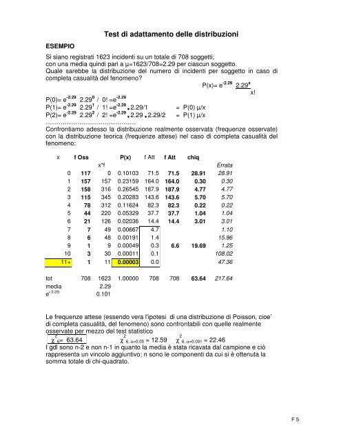
ESEMPIOTest di adattamento delle distribuzioniSi siano registrati 1623 incidenti su un totale di 708 soggetti;con una media quindi pari a µ=1623/708=2.29 per ciascun soggetto.Quale sarebbe la distribuzione del numero di incidenti per soggetto in caso dicompleta casualità del fenomeno?P(x)= e -2.29 2.29 xx!P(0)= e -2.29 2.29 0 / 0! =e -2.29P(1)= e -2.29 2.29 1 / 1! =e -2.29 ∗ 2.29/1 = P(0) µ/xP(2)= e -2.29 2.29 2 / 2! =e -2.29 ∗ 2.29 ∗ 2.29/2 = P(1) µ/x…………………………………….Confrontiamo adesso la distribuzione realmente osservata (frequenze osservate)con la distribuzione teorica (frequenze attese) nel caso di completa casualità delfenomeno:x f Oss P(x) f Att f Att chiqx*fErrata0 117 0 0.10103 71.5 71.5 28.91 28.911 157 157 0.23159 164.0 164.0 0.30 0.302 158 316 0.26545 187.9 187.9 4.77 4.773 115 345 0.20283 143.6 143.6 5.70 5.704 78 312 0.11624 82.3 82.3 0.22 0.225 44 220 0.05329 37.7 37.7 1.04 1.046 21 126 0.02036 14.4 14.4 3.01 3.017 7 49 0.00667 4.7 1.108 6 48 0.00191 1.4 15.969 1 9 0.00049 0.3 6.6 19.69 1.2510 3 30 0.00011 0.1 108.0211+ 1 11 0.00003 0.0 47.36tot 708 1623 1.00000 708 708 63.64 217.64media 2.29e (-2.29) 0.101Le frequenze attese (essendo vera l'ipotesi di una distribuzione di Poisson, cioe’di completa casualità, del fenomeno) sono confrontabili con quelle realmenteosservate per mezzo del test statisticoχ 2 6= 63.64 χ 2 6, α=0.05 = 12.59 χ 2 6, α=0.001 = 22.46I gdl sono n-2 e non n-1 in quanto la media è stata ricavata dal campione e ciòrappresenta un vincolo aggiuntivo; n sono le componenti da cui si è ottenuta lasomma totale di chi-quadrato.F 5