WIRELESS
Dynamic Channel Modeling at 2.4 GHz for On-Body Area Networks
Dynamic Channel Modeling at 2.4 GHz for On-Body Area Networks

You also want an ePaper? Increase the reach of your titles
YUMPU automatically turns print PDFs into web optimized ePapers that Google loves.
20 ADVANCES IN ELECTRONICS AND TELECOMMUNICATIONS, VOL. 2, NO. 4, DECEMBER 2011<br />
−20<br />
µ<br />
SA(µ)<br />
−40<br />
dB<br />
−60<br />
−80<br />
−100<br />
0 5 10 15 20 25 30 35 40<br />
Propagation distance [cm]<br />
(a) Mean µ<br />
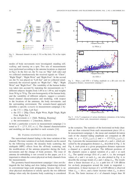
Fig. 3.<br />
[12]<br />
Measured channels in setup 2: TX on Hip (left), TX on Ear (right)<br />
7<br />
6<br />
5<br />
σ<br />
SA(σ)<br />
modes of body movements were investigated: standing still,<br />
walking, and running on a spot. Two sets of measurements<br />
were performed according to the antenna locations as depicted<br />
in Fig.3. In the first set, the Tx was on “Hip” (left side) and<br />
we collected simultaneously the received signals on “Chest”,<br />
“Right Thigh”, “Right Wrist” and “Right Foot”. In the second<br />
set, the Tx was placed on “Left Ear” and we collected simultaneously<br />
the received signals on “Right Ear”, “Hip”, ”Right<br />
Wrist” and ”Right Foot”. The variability of the human bodies<br />
was taken into account by repeating the measurements on 7<br />
different subjects: heights from 1.69 m to 1.89 m, and weights<br />
from 58 kg to 79 kg. The non-homogeneity of the human body,<br />
and the variability of different subjects, suggest a scenariobased<br />
channel characterization and modeling, with respect<br />
to the locations of the antennas, the body movements, and<br />
the surrounding environment. The scenario-based approach<br />
identifies a specific scenario in measurement campaign 2 by:<br />
• the T X ∈ {Hip, Left Ear}<br />
• the RX ∈ {Hip, Chest, Right Wrist, Right Thigh, Right<br />
Foot, Right Ear }<br />
• the movement m ∈ {Still, Walking, Running}<br />
• the environment e ∈ {Anechoic, Indoor}<br />
In brief, a particular scenario in measurement campaign 2 is<br />
noted as S = {T X, RX, m, e}. The channel characterization<br />
and modeling are then specified to each scenario [14].<br />
III. FADING STATISTICS AND MODELING<br />
The narrowband channel fading is the time-variation of the<br />
channel. The time-variation of on-body channels can be caused<br />
by the following reasons: the dynamic body scattering, the<br />
multipath (MPC) effects from the off-body scattering, and<br />
the modifications of the antenna properties during the body<br />
movements and the change of body postures. The issue of<br />
antenna de-embedding is not covered in this paper, yet it is<br />
important to obtain the correct physical on-body channels from<br />
the measurements.<br />
The geometry-based measurement campaign 1 does not distinguish<br />
the fast fading and slow fading (shadowing) defined<br />
in conventional large-scale propagation, because there is no<br />
clear physical mechanism to strictly specify the two different<br />
fadings when only the dynamic body scattering is considered<br />
dB<br />
4<br />
3<br />
2<br />
1<br />
0<br />
0 5 10 15 20 25 30 35 40<br />
Propagation distance [cm]<br />
(b) STD σ<br />
Fig. 4. Mean µ and STD σ of fading amplitude on a dB scale over the<br />
propagation distance, measurement campaign 1<br />
SA(χ 2 )<br />
5<br />
4<br />
3<br />
2<br />
1<br />
Lognormal<br />
Normal<br />
Nakagami<br />
Exponential<br />
Gamma<br />
Weibull<br />
Rayleigh<br />
Rice<br />
0<br />
0 5 10 15 20 25 30 35 40<br />
Propagation distance [cm]<br />
Fig. 5. SA[χ 2 ] comparison of various distribution estimations of the fading<br />
amplitude on a linear scale, measurement campaign 1<br />
in the scenarios. The statistics of the horizontal on-body channels<br />
are then extracted from each measurement piece (10 s).<br />
In measurement campaign 1, the mean and standard deviation<br />
(std) of the channel fading amplitude are computed on dB<br />
scale, i.e. µ = E[|S xy | dB (t n )] and σ = ST D[|S xy | dB (t n )].<br />
Fig. 4 presents the measurement results of µ and σ, which are<br />
sorted by the propagation distance d xy described in Fig. 2. In<br />
Fig. 4, each point at a given propagation distance represents<br />
a channel at a specific position. The different positions of<br />
the channels causes a spatial variation of µ and σ at each<br />
d xy . The spatial average (SA) of µ and σ, i.e. the averaged<br />
values of µ and σ at each d xy , are also plotted in Fig. 4, to<br />
describe the average trends of µ and σ along d xy . The results<br />
show a linear decrease of µ, i.e. a path loss of 1.68 dB/cm<br />
for on-body propagation around the trunk in tangential z-<br />
polarization. A linear increase of σ at 0.09 dB/cm is observed<br />
when d xy < 30cm, and a faster increase when d xy is above<br />
30 cm. The faster increase of σ of channels longer than 30


![1RUPDOQH \FLHFKU]H FLMD VNLH](https://img.yumpu.com/54031532/1/184x260/1rupdoqh-flhfkuh-flmd-vnlh.jpg?quality=85)