Unemployment cycles

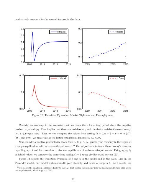
qualitatively accounts for the several features in the data.
0.6
0.5
θ Model
0.3
θ Data
0.4
0.2
0.3
0.2
0.1
0.1
2009 2011 2013 2015
2009 2011 2013 2015
0.15
u Model
0.15
u Data
0.1
0.1
0.05
0.05
2009 2011 2013 2015
2009 2011 2013 2015
Figure 12: Transition Dynamics: Market Tightness and Unemployment.
Consider an economy in the recession that has been there for a long period since the negative
productivity shock p 0 . That implies that the state variables u, γ and the choice variable θ are stationary,
i.e., ˙u, ˙γ, ˙θ equal zero. Then we can compute the values from setting Ω = 0, ˙u = ˙γ = ˙θ = 0 in (47),
(48), and (49). We treat this as the initial equilibrium denoted by u 0 , γ 0 , θ 0 .
Now consider a positive productivity shock from p 0 to p 1 > p h , pushing the economy in the region of
a unique equilibrium with active on-the-job search. 28 Our objective is to track the economy’s recovery
regarding u, γ, θ and its transition to the new equilibrium of active on-the-job search. Using u 0 , γ 0 , θ 0
as initial values, we compute the transitions setting Ω = 1 using the linearized system (23).
Figure 12 depicts the transition dynamics of θ and u in the model and in the data. Like in the
Pissarides model, our model features saddle path stability and hence a jump in θ. As a result, the
28 We choose the smallest possible productivity increase that pushes the economy into the unique equilibrium with active
on-the-job search, which is p 1 = 1.0262.
33