Unemployment cycles
WP201526
WP201526
You also want an ePaper? Increase the reach of your titles
YUMPU automatically turns print PDFs into web optimized ePapers that Google loves.
Dependence of cost on y. Let c(v) = c 0 vy. Then the first order conditions of both types of firms are given by:<br />
q(θ(Ω)) u s J 1 = c 0 y<br />
[ u<br />
q(θ(Ω))<br />
s J 1 + λ(Ω)γ ]<br />
J 2 ′ = c 0 y<br />
s<br />
Recall that we assume CRS, which is why both types of firms make on average zero profits (i.e. V = V =<br />
u<br />
0),<br />
[<br />
so that firms<br />
]<br />
are indifferent between posting low and high type vacancies. From the FOCs,<br />
s J 1y =<br />
u<br />
s J 1 + λ(Ω)γ<br />
s<br />
J 2 ′ y. We can then solve this equation for m(θ) (and, assuming the telegraph matching function,<br />
also for θ) as a function of π.<br />
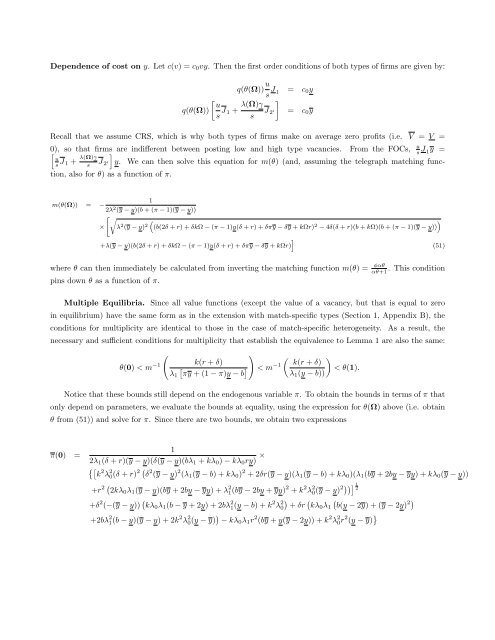
1<br />
m(θ(Ω)) = −<br />
2λ 2 (y − y)(b + (π − 1)(y − y))<br />
[√<br />
)<br />
× λ 2 (y − y)<br />
((b(2δ 2 + r) + δkΩ − (π − 1)y(δ + r) + δπy − δy + kΩr) 2 − 4δ(δ + r)(b + kΩ)(b + (π − 1)(y − y))<br />
]<br />
+λ(y − y)(b(2δ + r) + δkΩ − (π − 1)y(δ + r) + δπy − δy + kΩr)<br />
(51)<br />
where θ can then immediately be calculated from inverting the matching function m(θ) = φαθ<br />
αθ+1<br />
. This condition<br />
pins down θ as a function of π.<br />
Multiple Equilibria. Since all value functions (except the value of a vacancy, but that is equal to zero<br />
in equilibrium) have the same form as in the extension with match-specific types (Section 1, Appendix B), the<br />
conditions for multiplicity are identical to those in the case of match-specific heterogeneity.<br />
As a result, the<br />
necessary and sufficient conditions for multiplicity that establish the equivalence to Lemma 1 are also the same:<br />
(<br />
)<br />
θ(0) < m −1 k(r + δ)<br />
[ ]<br />
λ 1 πy + (1 − π)y − b<br />
( ) k(r + δ)<br />
< m −1 < θ(1).<br />
λ 1 (y − b))<br />
Notice that these bounds still depend on the endogenous variable π. To obtain the bounds in terms of π that<br />
only depend on parameters, we evaluate the bounds at equality, using the expression for θ(Ω) above (i.e. obtain<br />
θ from (51)) and solve for π. Since there are two bounds, we obtain two expressions<br />
π(0) =<br />
1<br />
2λ 1 (δ + r)(y − y)(δ(y − y)(bλ 1 + kλ 0 ) − kλ 0 ry) ×<br />
{[<br />
k 2 λ 2 0(δ + r) 2 ( δ 2 (y − y) 2 (λ 1 (y − b) + kλ 0 ) 2 + 2δr(y − y)(λ 1 (y − b) + kλ 0 )(λ 1 (by + 2by − yy) + kλ 0 (y − y))<br />
+r 2 ( 2kλ 0 λ 1 (y − y)(by + 2by − yy) + λ 2 1(by − 2by + yy) 2 + k 2 λ 2 0(y − y) 2))] 1 2<br />
+δ 2 (−(y − y)) ( kλ 0 λ 1 (b − y + 2y) + 2bλ 2 1(y − b) + k 2 λ 2 ) ( (<br />
0 + δr kλ0 λ 1 b(y − 2y) + (y − 2y)<br />
2 )<br />
+2bλ 2 1(b − y)(y − y) + 2k 2 λ 2 0(y − y) ) − kλ 0 λ 1 r 2 (by + y(y − 2y)) + k 2 λ 2 0r 2 (y − y) }


