Unemployment cycles

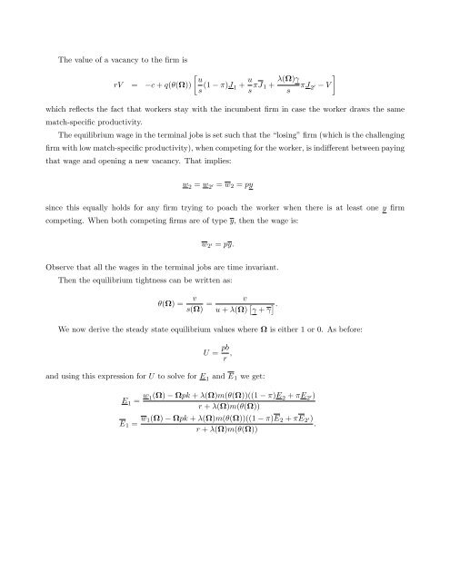
The value of a vacancy to the firm is
[ u
rV = −c + q(θ(Ω))
s (1 − π)J 1 + u s πJ 1 + λ(Ω)γ ]
πJ
s 2 ′ − V
which reflects the fact that workers stay with the incumbent firm in case the worker draws the same
match-specific productivity.
The equilibrium wage in the terminal jobs is set such that the “losing” firm (which is the challenging
firm with low match-specific productivity), when competing for the worker, is indifferent between paying
that wage and opening a new vacancy. That implies:
w 2 = w 2 ′ = w 2 = py
since this equally holds for any firm trying to poach the worker when there is at least one y firm
competing. When both competing firms are of type y, then the wage is:
w 2 ′ = py.
Observe that all the wages in the terminal jobs are time invariant.
Then the equilibrium tightness can be written as:
θ(Ω) =
v
s(Ω) =
v
u + λ(Ω) [ γ + γ ].
We now derive the steady state equilibrium values where Ω is either 1 or 0. As before:
U = pb
r ,
and using this expression for U to solve for E 1 and E 1 we get:
E 1 = w 1(Ω) − Ωpk + λ(Ω)m(θ(Ω))((1 − π)E 2 + πE 2 ′)
r + λ(Ω)m(θ(Ω))
E 1 = w 1(Ω) − Ωpk + λ(Ω)m(θ(Ω))((1 − π)E 2 + πE 2 ′)
.
r + λ(Ω)m(θ(Ω))