Introduction to Relativistic Quantum Field Theory - Frankfurt Institute ...
Introduction to Relativistic Quantum Field Theory - Frankfurt Institute ...
Introduction to Relativistic Quantum Field Theory - Frankfurt Institute ...

Create successful ePaper yourself
Turn your PDF publications into a flip-book with our unique Google optimized e-Paper software.
1 e-mail: hees@fias.uni-frankfurt.de<br />
<strong>Introduction</strong> <strong>to</strong><br />
<strong>Relativistic</strong> <strong>Quantum</strong> <strong>Field</strong> <strong>Theory</strong><br />
Hendrik van Hees 1<br />
Goethe-Universität <strong>Frankfurt</strong><br />
<strong>Frankfurt</strong> Insitute for Advanced Studies<br />
D-60438 <strong>Frankfurt</strong> am Main<br />
Germany<br />
31st Oc<strong>to</strong>ber 2012
Contents<br />
1 Path Integrals 11<br />
1.1 <strong>Quantum</strong> Mechanics . . . . . . . . . . . . . . . . . . . . . . . . . . . . . . . . . . . . 11<br />
1.2 Choice of the Picture . . . . . . . . . . . . . . . . . . . . . . . . . . . . . . . . . . . . 14<br />
1.3 Formal Solution of the Equations of Motion . . . . . . . . . . . . . . . . . . . . . . . 16<br />
1.4 Example: The Free Particle . . . . . . . . . . . . . . . . . . . . . . . . . . . . . . . . 18<br />
1.5 The Feynman-Kac Formula . . . . . . . . . . . . . . . . . . . . . . . . . . . . . . . . 20<br />
1.6 The Path Integral for the Harmonic Oscilla<strong>to</strong>r . . . . . . . . . . . . . . . . . . . . . . 24<br />
1.7 Some Rules for Path Integrals . . . . . . . . . . . . . . . . . . . . . . . . . . . . . . . 27<br />
1.8 The Schrödinger Wave Equation . . . . . . . . . . . . . . . . . . . . . . . . . . . . . 27<br />
1.9 Potential Scattering . . . . . . . . . . . . . . . . . . . . . . . . . . . . . . . . . . . . 29<br />
1.10 Generating functional for Vacuum Expectation Values . . . . . . . . . . . . . . . . . 35<br />
1.11 Bosons and Fermions, and what else? . . . . . . . . . . . . . . . . . . . . . . . . . . . 37<br />
2 Nonrelativistic Many-Particle <strong>Theory</strong> 39<br />
2.1 The Fock Space Representation of <strong>Quantum</strong> Mechanics . . . . . . . . . . . . . . . . 39<br />
3 Canonical <strong>Field</strong> Quantisation 43<br />
3.1 Space and Time in Special Relativity . . . . . . . . . . . . . . . . . . . . . . . . . . . 44<br />
3.2 Tensors and Scalar <strong>Field</strong>s . . . . . . . . . . . . . . . . . . . . . . . . . . . . . . . . . 48<br />
3.3 Noether’s Theorem (Classical Part) . . . . . . . . . . . . . . . . . . . . . . . . . . . . 53<br />
3.4 Canonical Quantisation . . . . . . . . . . . . . . . . . . . . . . . . . . . . . . . . . . 58<br />
3.5 The Most Simple Interacting <strong>Field</strong> <strong>Theory</strong>: φ 4 . . . . . . . . . . . . . . . . . . . . . 64<br />
3.6 The LSZ Reduction Formula . . . . . . . . . . . . . . . . . . . . . . . . . . . . . . . 66<br />
3.7 The Dyson-Wick Series . . . . . . . . . . . . . . . . . . . . . . . . . . . . . . . . . . 67<br />
3.8 Wick’s Theorem . . . . . . . . . . . . . . . . . . . . . . . . . . . . . . . . . . . . . . 69<br />
3.9 The Feynman Diagrams . . . . . . . . . . . . . . . . . . . . . . . . . . . . . . . . . . 72<br />
3
Contents<br />
4 <strong>Relativistic</strong> <strong>Quantum</strong> <strong>Field</strong>s 79<br />
4.1 Causal Massive <strong>Field</strong>s . . . . . . . . . . . . . . . . . . . . . . . . . . . . . . . . . . . 80<br />
4.1.1 Massive Vec<strong>to</strong>r <strong>Field</strong>s . . . . . . . . . . . . . . . . . . . . . . . . . . . . . . . 81<br />
4.1.2 Massive Spin-1/2 <strong>Field</strong>s . . . . . . . . . . . . . . . . . . . . . . . . . . . . . . 82<br />
4.2 Causal Massless <strong>Field</strong>s . . . . . . . . . . . . . . . . . . . . . . . . . . . . . . . . . . . 86<br />
4.2.1 Massless Vec<strong>to</strong>r <strong>Field</strong> . . . . . . . . . . . . . . . . . . . . . . . . . . . . . . . 86<br />
4.2.2 Massless Helicity 1/2 <strong>Field</strong>s . . . . . . . . . . . . . . . . . . . . . . . . . . . . 89<br />
4.3 Quantisation and the Spin-Statistics Theorem . . . . . . . . . . . . . . . . . . . . . . 89<br />
4.3.1 Quantisation of the spin-1/2 Dirac <strong>Field</strong> . . . . . . . . . . . . . . . . . . . . . 90<br />
4.4 Discrete Symmetries and the CP T Theorem . . . . . . . . . . . . . . . . . . . . . . . 94<br />
4.4.1 Charge Conjugation for Dirac spinors . . . . . . . . . . . . . . . . . . . . . . 94<br />
4.4.2 Time Reversal . . . . . . . . . . . . . . . . . . . . . . . . . . . . . . . . . . . 96<br />
4.4.3 Parity . . . . . . . . . . . . . . . . . . . . . . . . . . . . . . . . . . . . . . . . 98<br />
4.4.4 Lorentz Classification of Bilinear Forms . . . . . . . . . . . . . . . . . . . . . 98<br />
4.4.5 The CP T Theorem . . . . . . . . . . . . . . . . . . . . . . . . . . . . . . . . 100<br />
4.4.6 Remark on Strictly Neutral Spin–1/2–Fermions . . . . . . . . . . . . . . . . . 102<br />
4.5 Path Integral Formulation . . . . . . . . . . . . . . . . . . . . . . . . . . . . . . . . . 103<br />
4.5.1 Example: The Free Scalar <strong>Field</strong> . . . . . . . . . . . . . . . . . . . . . . . . . . 109<br />
4.5.2 The Feynman Rules for φ 4 revisited . . . . . . . . . . . . . . . . . . . . . . . 111<br />
4.6 Generating Functionals . . . . . . . . . . . . . . . . . . . . . . . . . . . . . . . . . . . 113<br />
4.6.1 LSZ Reduction . . . . . . . . . . . . . . . . . . . . . . . . . . . . . . . . . . . 114<br />
4.6.2 The equivalence theorem . . . . . . . . . . . . . . . . . . . . . . . . . . . . . 115<br />
4.6.3 Generating Functional for Connected Green’s Functions . . . . . . . . . . . . 116<br />
4.6.4 Effective Action and Vertex Functions . . . . . . . . . . . . . . . . . . . . . . 119<br />
4.6.5 Noether’s Theorem (<strong>Quantum</strong> Part) . . . . . . . . . . . . . . . . . . . . . . . 123<br />
4.6.6 �-Expansion . . . . . . . . . . . . . . . . . . . . . . . . . . . . . . . . . . . . . 125<br />
4.7 A Simple Interacting <strong>Field</strong> <strong>Theory</strong> with Fermions . . . . . . . . . . . . . . . . . . . . 129<br />
5 Renormalisation 135<br />
5.1 Infinities and how <strong>to</strong> cure them . . . . . . . . . . . . . . . . . . . . . . . . . . . . . . 135<br />
5.1.1 Overview over the renormalisation procedure . . . . . . . . . . . . . . . . . . 139<br />
5.2 Wick rotation . . . . . . . . . . . . . . . . . . . . . . . . . . . . . . . . . . . . . . . . 141<br />
5.3 Dimensional regularisation . . . . . . . . . . . . . . . . . . . . . . . . . . . . . . . . . 145<br />
5.3.1 The Γ-function . . . . . . . . . . . . . . . . . . . . . . . . . . . . . . . . . . . 146<br />
5.3.2 Spherical coordinates in d dimensions . . . . . . . . . . . . . . . . . . . . . . 153<br />
4
Contents<br />
5.3.3 Standard-integrals for Feynman integrals . . . . . . . . . . . . . . . . . . . . 154<br />
5.4 The 4-point vertex correction at 1-loop order . . . . . . . . . . . . . . . . . . . . . . 157<br />
5.5 Power counting . . . . . . . . . . . . . . . . . . . . . . . . . . . . . . . . . . . . . . . 159<br />
5.6 The setting-sun diagram . . . . . . . . . . . . . . . . . . . . . . . . . . . . . . . . . . 162<br />
5.7 Weinberg’s Theorem . . . . . . . . . . . . . . . . . . . . . . . . . . . . . . . . . . . . 166<br />
5.7.1 Proof of Weinberg’s theorem . . . . . . . . . . . . . . . . . . . . . . . . . . . 169<br />
5.7.2 Proof of the Lemma . . . . . . . . . . . . . . . . . . . . . . . . . . . . . . . . 176<br />
5.8 Application of Weinberg’s Theorem <strong>to</strong> Feynman diagrams . . . . . . . . . . . . . . . 178<br />
5.9 BPH-Renormalisation . . . . . . . . . . . . . . . . . . . . . . . . . . . . . . . . . . . 181<br />
5.9.1 Some examples of the method . . . . . . . . . . . . . . . . . . . . . . . . . . . 182<br />
5.9.2 The general BPH-formalism . . . . . . . . . . . . . . . . . . . . . . . . . . . . 184<br />
5.10 Zimmermann’s forest formula . . . . . . . . . . . . . . . . . . . . . . . . . . . . . . . 186<br />
5.11 Global linear symmetries and renormalisation . . . . . . . . . . . . . . . . . . . . . . 189<br />
5.11.1 Example: 1-loop renormalisation . . . . . . . . . . . . . . . . . . . . . . . . . 194<br />
5.12 Renormalisation group equations . . . . . . . . . . . . . . . . . . . . . . . . . . . . . 197<br />
5.12.1 Homogeneous RGEs and modified BPHZ renormalisation . . . . . . . . . . . 198<br />
5.12.2 The homogeneous RGE and dimensional regularisation . . . . . . . . . . . . . 201<br />
5.12.3 Solutions <strong>to</strong> the homogeneous RGE . . . . . . . . . . . . . . . . . . . . . . . 202<br />
5.12.4 Independence of the S-Matrix from the renormalisation scale . . . . . . . . . 203<br />
5.13 Asymp<strong>to</strong>tic behaviour of vertex functions . . . . . . . . . . . . . . . . . . . . . . . . 204<br />
5.13.1 The Gell-Mann-Low equation . . . . . . . . . . . . . . . . . . . . . . . . . . . 205<br />
5.13.2 The Callan-Symanzik equation . . . . . . . . . . . . . . . . . . . . . . . . . . 206<br />
6 <strong>Quantum</strong> Electrodynamics 211<br />
6.1 Gauge <strong>Theory</strong> . . . . . . . . . . . . . . . . . . . . . . . . . . . . . . . . . . . . . . . . 211<br />
6.2 Matter <strong>Field</strong>s interacting with Pho<strong>to</strong>ns . . . . . . . . . . . . . . . . . . . . . . . . . . 217<br />
6.3 Canonical Path Integral . . . . . . . . . . . . . . . . . . . . . . . . . . . . . . . . . . 220<br />
6.4 Invariant Cross Sections . . . . . . . . . . . . . . . . . . . . . . . . . . . . . . . . . . 224<br />
6.5 Tree level calculations of some physical processes . . . . . . . . . . . . . . . . . . . . 227<br />
6.5.1 Comp<strong>to</strong>n Scattering . . . . . . . . . . . . . . . . . . . . . . . . . . . . . . . . 228<br />
6.5.2 Annihilation of an e − e + -pair . . . . . . . . . . . . . . . . . . . . . . . . . . . 231<br />
6.6 The Background <strong>Field</strong> Method . . . . . . . . . . . . . . . . . . . . . . . . . . . . . . 233<br />
6.6.1 The background field method for non-gauge theories . . . . . . . . . . . . . . 233<br />
6.6.2 Gauge theories and background fields . . . . . . . . . . . . . . . . . . . . . . 234<br />
6.6.3 Renormalisability of the effective action in background field gauge . . . . . . 237<br />
5
Contents<br />
7 Nonabelian Gauge fields 241<br />
7.1 The principle of local gauge invariance . . . . . . . . . . . . . . . . . . . . . . . . . . 241<br />
7.2 Quantisation of nonabelian gauge field theories . . . . . . . . . . . . . . . . . . . . . 245<br />
7.2.1 BRST-Invariance . . . . . . . . . . . . . . . . . . . . . . . . . . . . . . . . . . 247<br />
7.2.2 Gauge independence of the S-matrix . . . . . . . . . . . . . . . . . . . . . . . 251<br />
7.3 Renormalisability of nonabelian gauge theories in BFG . . . . . . . . . . . . . . . . . 253<br />
7.3.1 The symmetry properties in the background field gauge . . . . . . . . . . . . 253<br />
7.3.2 The BFG Feynman rules . . . . . . . . . . . . . . . . . . . . . . . . . . . . . 256<br />
7.4 Renormalisability of nonabelian gauge theories (BRST) . . . . . . . . . . . . . . . . 259<br />
7.4.1 The Ward-Takahashi identities . . . . . . . . . . . . . . . . . . . . . . . . . . 259<br />
A Variational Calculus and Functional Methods 263<br />
A.1 The Fundamental Lemma of Variational Calculus . . . . . . . . . . . . . . . . . . . . 263<br />
A.2 Functional Derivatives . . . . . . . . . . . . . . . . . . . . . . . . . . . . . . . . . . . 265<br />
B The Symmetry of Space and Time 269<br />
B.1 The Lorentz Group . . . . . . . . . . . . . . . . . . . . . . . . . . . . . . . . . . . . . 269<br />
B.2 Representations of the Lorentz Group . . . . . . . . . . . . . . . . . . . . . . . . . . 276<br />
B.3 Representations of the Full Lorentz Group . . . . . . . . . . . . . . . . . . . . . . . . 278<br />
B.4 Unitary Representations of the Poincaré Group . . . . . . . . . . . . . . . . . . . . . 281<br />
B.4.1 The Massive States . . . . . . . . . . . . . . . . . . . . . . . . . . . . . . . . . 285<br />
B.4.2 Massless Particles . . . . . . . . . . . . . . . . . . . . . . . . . . . . . . . . . 287<br />
B.5 The Invariant Scalar Product . . . . . . . . . . . . . . . . . . . . . . . . . . . . . . . 289<br />
C Formulae 291<br />
C.1 Amplitudes for various free fields . . . . . . . . . . . . . . . . . . . . . . . . . . . . . 291<br />
C.2 Dimensional regularised Feynman-integrals . . . . . . . . . . . . . . . . . . . . . . . 292<br />
C.3 Laurent expansion of the Γ-Function . . . . . . . . . . . . . . . . . . . . . . . . . . . 292<br />
C.4 Feynman’s Parameterisation . . . . . . . . . . . . . . . . . . . . . . . . . . . . . . . . 293<br />
Bibliography 295<br />
6
Preface<br />
The following is a script, which tries <strong>to</strong> collect and extend some ideas about <strong>Quantum</strong> <strong>Field</strong> <strong>Theory</strong><br />
for the International Student Programs at GSI.<br />
In the first chapter, we start with some facts known, from ordinary nonrelativistic quantum mechanics.<br />
We emphasise the picture of the evolution of quantum systems in space and time. The<br />
aim was <strong>to</strong> introduce the functional methods of path integrals on hand of the familiar framework<br />
of nonrelativistic quantum theory.<br />
In this introduc<strong>to</strong>ry chapter it was my goal <strong>to</strong> keep the s<strong>to</strong>ry as simple as possible. Thus, all<br />
problems concerning opera<strong>to</strong>r ordering or interaction with electromagnetic fields were omitted. All<br />
these <strong>to</strong>pics will be treated in terms of quantum field theory, beginning with the third chapter.<br />
The second chapter is not yet written completely. It will be short and is intended <strong>to</strong> contain the<br />
vacuum many-body theory for nonrelativistic particles given as a quantum many-particle theory. It<br />
is shown that the same theory can be obtained by using the field-quantisation method (which was<br />
often called “the second quantisation”, but on my opinion this is a very misleading term). I intend<br />
<strong>to</strong> work out the most simple applications <strong>to</strong> the hydrogen a<strong>to</strong>m including bound states and exact<br />
scattering theory.<br />
In the third chapter, we start with the classical principles of special relativity which are Lorentz<br />
covariance and the action principle in the covariant Lagrangian formulation, but we shall introduce<br />
only scalar fields <strong>to</strong> keep the stuff quite easy, since there is only one field degree of freedom. The<br />
classical part of the chapter ends with a discussion of Noether’s theorem which is on the heart of<br />
our approach <strong>to</strong> observables which are defined from conserved currents caused by symmetries of<br />
space and time as well as by intrinsic symmetries of the fields.<br />
After that introduction <strong>to</strong> classical relativistic field theory, we quantise the free fields, ending with<br />
a sketch about the nowadays well established facts of relativistic quantum theory: It is necessarily<br />
a many-body theory, because there is no possibility for a Schrödinger-like one-particle theory. The<br />
physical reason is simply the possibility of creation and annihilation of particle-antiparticle pairs<br />
(pair creation). It will come out that for a local quantum field theory the Hamil<strong>to</strong>nian of the free<br />
particles is bounded from below for the quantised field theory only if we quantise it with bosonic<br />
commutation relations. This is a special case of the famous spin-statistics theorem.<br />
Then we show, how <strong>to</strong> treat φ 4 theory as the most simple example of an interacting field theory<br />
with help of perturbation theory, prove Wick’s theorem and the LSZ-reduction formula. The goal<br />
of this chapter is a derivation of the perturbative Feynman-diagram rules. The chapter ends with<br />
the sad result that diagrams, which contain loops, correspond <strong>to</strong> integrals which do not exist since<br />
7
Preface<br />
they are divergent. This difficulty is solved by renormalisation theory which will be treated later in<br />
these notes.<br />
The fourth chapter starts with a systematic treatment of relativistic invariant theory using appendix<br />
B which contains the complete mathematical treatment of the representation theory of the Poincaré<br />
group, as far as it is necessary for physics. The most important result is the general proof of the<br />
spin-statistics theorem and the PCT theorem.<br />
The rest of the chapter contains the foundations of path integrals for quantum field theories. Hereby,<br />
we shall find the methods helpful, which we have learnt in Chapter 1. This contains also the path<br />
integral formalism for fermions which needs a short introduction <strong>to</strong> the mathematics of Grassmann<br />
numbers.<br />
After setting up these facts, we shall rederive the perturbation theory, which we have found with<br />
help of Wick’s theorem in chapter 3 from the opera<strong>to</strong>r formalism. We shall use from the very<br />
beginning the diagrams as a very intuitive technique for book-keeping of the rather technically<br />
involved functional derivatives of the generating functional for Green’s functions. On the other<br />
hand we shall also illustrate the ,,digram-less” derivation of the �-expansion which corresponds <strong>to</strong><br />
the number of loops in the diagrams.<br />
We shall also give a complete proof of the theorems about generating functionals for subclasses of<br />
diagrams, namely the connected Green’s functions and the proper vertex functions.<br />
The chapter ends with the derivation of the Feynman rules for a simple <strong>to</strong>y theory involving a Dirac<br />
spin 1/2 Fermi field with the now completely developed functional (path integral) technique. As<br />
will come out quite straight forwardly, the only difference compared <strong>to</strong> the pure boson case are some<br />
sign rules for fermion lines and diagrams containing a closed fermion loop, coming from the fact that<br />
we have anticommuting Grassmann numbers for the fermions rather than commuting c-numbers<br />
for the bosons.<br />
Chapter 5 is a detailed treatment of modern renormalisation theory. Here, we emphasise the<br />
calculation techniques, needed <strong>to</strong> calculate Feynman diagrams which have <strong>to</strong> be regularised in some<br />
way. I have chosen dimensional regularisation from the very beginning, because it leads <strong>to</strong> the most<br />
convenient treatment which is espacially true for the physically most important gauge field theories,<br />
about which we will learn in the later chapters of these notes. We will also prove Weinberg’s theorem<br />
and the finiteness of the renormalised diagrams within the BPHZ formalism.<br />
The sixth chapter is devoted <strong>to</strong> QED, including the most simple physical applications at tree-level.<br />
From the very beginning we shall take the gauge theoretical point of view. Gauge theories have<br />
proved <strong>to</strong> be the most important class of field theories, including the Standard Model of elementary<br />
particles. Thus, we use from the very beginning the modern techniques <strong>to</strong> quantise the theory<br />
with help of formal path integral manipulations, known as Faddeev-Popov quantisation in a certain<br />
class of covariant gauges. We shall also derive the very important Ward-Takahashi identities. As<br />
an especially useful gauge fixing we shall also formulate the background field gauge which is a<br />
manifestly gauge invariant procedure. We shall give the proof of renormalisability of QED in the<br />
background field gauge.<br />
Chapter 7 contains a complete treatment of nonabelian gauge theories, including the notion of<br />
BRST invariance and renormalisability of these type of theories.<br />
8
Preface<br />
The appendix contains some mathematical material needed in the main parts.<br />
Appendix A introduces some very basic facts about functionals and variational calculus.<br />
Appendix B has grown a little lengthy, but on the other hand I think it is useful <strong>to</strong> write down<br />
all the stuff about the representation theory of the Poincaré groups. In a way it may be seen as a<br />
simplification of Wigner’s famous paper from 1939.<br />
Appendix C I hope the reader of my notes will have as much fun as I had when I wrote them!<br />
Last but not least I come <strong>to</strong> the acknowledgements. First <strong>to</strong> mention are Robert Roth and Chris<strong>to</strong>ph<br />
Appel who gave me their various book style hackings for making it as nice looking as it is.<br />
Also Thomas Neff has contributed by his patient help with all “mysteries” of the computer systems,<br />
I used at GSI, while I prepared this script.<br />
Chris<strong>to</strong>ph Appel was always discussing with me about the hot <strong>to</strong>pics of QFT, like, e.g., obtaining<br />
the correct symmetry fac<strong>to</strong>rs of diagrams and the proper use of Feynman rules for various types of<br />
QFTs. He was also carefully reading the script and has corrected many spelling errors.<br />
Literature<br />
Finally I have <strong>to</strong> stress the fact that the lack of citations in these notes mean not that I claim that<br />
the contents are original ideas of mine. It was just my laziness in finding out all the references I<br />
used through my own <strong>to</strong>ur through the literature and learning of quantum field theory.<br />
I just cite some of the textbooks I found most illuminating during the preparation of these notes: For<br />
the fundamentals there exist a lot of textbooks of very different quality. For me the most important<br />
were [PS95, Wei95, Wei96, Kak93, Kug97]. Concerning gauge theories some of the clearest sources<br />
of textbook or review character are [Tay76, AL73, FLS72, Kug97, LZJ72a, LZJ72b, LZJ72c]. One<br />
of the most difficult <strong>to</strong>pics in quantum field theory is the question of renormalisation. Except the<br />
already mentioned textbooks, here I found the original papers very important, some of them are<br />
[BP57, Wei60, Zim68, Zim69, Zim70]. A very nice and concise monograph of this <strong>to</strong>pic is [Col86].<br />
Whenever I was aware of a URL with the full text of the paper, I cited it <strong>to</strong>o, so that one can access<br />
these papers as easily as possible.<br />
9
Preface<br />
10
Chapter 1<br />
Path Integrals<br />
In this chapter we shall summarise some well known facts about nonrelativistic quantum mechanics<br />
in terms of path integrals, which where invented by Feynman in 1948 as an alternative formulation<br />
of quantum mechanics. It is thought <strong>to</strong> be an introduction <strong>to</strong> the <strong>to</strong>ols of functional methods used<br />
in quantum field theory.<br />
1.1 <strong>Quantum</strong> Mechanics<br />
In this course we assume that the reader is familiar with quantum mechanics in terms of Dirac’s<br />
bra- and ket formalism. We repeat the basic facts by giving some postulates about the structure of<br />
quantum mechanics which are valid in the nonrelativistic case as well as in the relativistic. In these<br />
notes, we emphasise that quantum theory is the description of physical systems in space and time.<br />
As we know, this picture is in some sense valid for a wider range of phenomena than the classical<br />
picture of particles and fields.<br />
Although it is an interesting <strong>to</strong>pic, we do not care about some problems with philosophy of quantum<br />
mechanics. In my opinion, the physicists have a well unders<strong>to</strong>od way in applying the formalism <strong>to</strong><br />
phenomena in nature, and the problem of measurement is not of practical physical importance. That<br />
sight seems <strong>to</strong> be settled by all experimental tests of quantum theory, undertaken so far: They all<br />
show that quantum theory is correct in predicting and explaining the outcome of experiments with<br />
systems and there is no (practical) problem in interpreting the results from calculating “physical<br />
properties of systems” with help of the formalism given by the mathematical <strong>to</strong>ol “quantum theory”.<br />
So let us begin with the summary of the mathematical structure of quantum mechanics, as it is<br />
formulated in Dirac’s famous book.<br />
• Each quantum system is described completely by a ray in a Hilbert space H . A ray is defined<br />
as the following equivalence class of vec<strong>to</strong>rs:<br />
[|ψ〉] = {c |ψ〉 | |ψ〉 ∈ H , c ∈ C \ {0}}. (1.1)<br />
If the system is in a certain state [|ψ1〉], then the probability <strong>to</strong> find it in the state [|ψ2〉] is<br />
11
given by<br />
Chapter 1 · Path Integrals<br />
| 〈ψ1 | ψ2 〉 |<br />
P12 =<br />
2<br />
. (1.2)<br />
〈ψ1 | ψ1 〉 〈ψ2 | ψ2 〉<br />
• The observables of the system are represented by selfadjoint opera<strong>to</strong>rs O which build <strong>to</strong>gether<br />
with the unity opera<strong>to</strong>r an algebra of opera<strong>to</strong>rs, acting on the Hilbert-space vec<strong>to</strong>rs. For<br />
instance, in the case of a quantised classical point particle this algebra of observables is built by<br />
the opera<strong>to</strong>rs of the Cartesian components of position and (canonical) momentum opera<strong>to</strong>rs,<br />
which fulfil the Heisenberg algebra:<br />
[xi, xk] = [p i, p k] = 0, [xi, p k] = iδik1. (1.3)<br />
Here and further on (except in cases when it is stated explicitly) we set Planck’s constant<br />
� = 1. In the next chapter, when we look on relativity, we shall set the velocity of light c = 1<br />
<strong>to</strong>o. In this so called natural system of units, observables with the dimension of an action are<br />
dimensionless. Spatial distances and time intervals have the same unit which is reciprocal <strong>to</strong><br />
that of energy and momentum, and convenient unities in particle physics are MeV or GeV<br />
for energies, momenta and masses and fm for space or time intervals. The conversion within<br />
these units is given by the value �c � 0.197 GeV fm.<br />
A possible result of a precise measurement of the observable O is necessarily an eigenvalue<br />
of the corresponding opera<strong>to</strong>r O. Because O is selfadjoint, its eigenvalues are real, and the<br />
eigenvec<strong>to</strong>rs can be chosen such that they build a complete normalised set of kets. After an<br />
ideal measurement, the system is in an eigenket with the measured eigenvalue.<br />
The most famous consequence of this description of physical systems is Heisenberg’s uncertainty<br />
relation, which follows from the positive definiteness of the scalar product in Hilbert<br />
space:<br />
∆A∆B ≥ 1<br />
|〈[A, B]〉| . (1.4)<br />
2<br />
Two observables are simultaneously exactly measurable if and only if the corresponding opera<strong>to</strong>rs<br />
commute. In this case both opera<strong>to</strong>rs have common eigenvec<strong>to</strong>rs. After a simultaneous<br />
measurement, the system is in a corresponding common eigenstate.<br />
A set of pairwise commutating observables is said <strong>to</strong> be complete if the simultaneous measurement<br />
of all these observables fixes the state of the system completely, i.e., if the simultaneous<br />
eigenspaces of these opera<strong>to</strong>rs are one-dimensional (nondegenerate).<br />
• Time is represented by a real parameter. There is an hermitian opera<strong>to</strong>r H, associated with<br />
the system such that, if O is an observable, then<br />
is the opera<strong>to</strong>r of the time derivative of this observable.<br />
˚O = 1<br />
i [O, H] + ∂tO (1.5)<br />
The partial time derivative is only for the explicit time dependence. The fundamental opera<strong>to</strong>rs<br />
like space and momentum opera<strong>to</strong>rs, which form a complete generating system of the<br />
12
1.1 · <strong>Quantum</strong> Mechanics<br />
algebra of observables, are not explicitly time dependent (by definition!). It should be emphasised<br />
that ˚ O is usually not the mathematical <strong>to</strong>tal derivative with respect <strong>to</strong> time. We shall<br />
see that the mathematical dependence on time is arbitrary in a wide sense, because, if we have<br />
a description of quantum mechanics, then we are free <strong>to</strong> transform the opera<strong>to</strong>rs and state<br />
kets by a time dependent unitary transformation without changing any physical prediction<br />
(probabilities, mean values of observables etc.).<br />
• Due <strong>to</strong> our first assumption, the state of the quantum system is completely known, if we<br />
know a state ket |ψ〉 lying in the ray [|ψ〉], in which the system is prepared in, at an arbitrary<br />
initial time. This preparation of a system is possible by performing a precise simultaneous<br />
measurement of a complete set of compatible observables.<br />
It is more convenient <strong>to</strong> have a description of the state in terms of Hilbert-space quantities<br />
than in terms of the projective space (built by the above defined rays). It is easy <strong>to</strong> see that<br />
the state is uniquely given by the projection opera<strong>to</strong>r<br />
P |ψ〉 =<br />
|ψ〉 〈ψ|<br />
, (1.6)<br />
�ψ�2 with |ψ〉 an arbitrary ket contained in the ray (i.e., the state the system is in).<br />
• In general, especially if we like <strong>to</strong> describe macroscopic systems within quantum mechanics,<br />
we do not know the state of the system completely. In this case, we can describe the system<br />
by a selfadjoint statistical opera<strong>to</strong>r ρ which is positive semidefinite (that means that for all<br />
kets |ψ〉 ∈ H we have 〈ψ |ρ| ψ〉 ≥ 0) and fulfils the normalisation condition Tr ρ = 1. It is<br />
chosen so that it is consistent with the knowledge about the system we have and contains no<br />
more information than one really has. This concept will be explained in a later section.<br />
The trace of an opera<strong>to</strong>r is defined with help of a complete set of orthonormal vec<strong>to</strong>rs |n〉 as<br />
Tr ρ = �<br />
n 〈n |ρ| n〉. The mean value of any opera<strong>to</strong>r O is given by 〈O〉 = Tr(Oρ).<br />
The meaning of the statistical opera<strong>to</strong>r is easily seen from these definitions. Since the opera<strong>to</strong>r<br />
P |n〉 answers the question, whether the system is in the state [|n〉] the probability that the<br />
system is in the state [|n〉] is given by pn = Tr(P |n〉ρ) = 〈n |ρ| n〉. If |n〉 is given as the complete<br />
set of eigenvec<strong>to</strong>rs of an observable opera<strong>to</strong>r O for the eigenvalues On, then the mean value<br />
of O is 〈O〉 = �<br />
n pnOn in agreement with the fundamental definition of the expectation<br />
value of a s<strong>to</strong>chastic variable in dependence of the given probabilities for the outcome of a<br />
measurement of this variable.<br />
The last assumption of quantum theory is that the statistical opera<strong>to</strong>r is given for the system<br />
at all times. This requires that<br />
˚ρ = 1<br />
i [ρ, H] + ∂tρ = 0. (1.7)<br />
This equation is also valid for the special case that the system is in a pure state, i.e. for<br />
ρ = P |ψ〉.<br />
13
1.2 Choice of the Picture<br />
Chapter 1 · Path Integrals<br />
Now, having briefly summarised how quantum mechanics works, we like <strong>to</strong> give the time evolution a<br />
mathematical content, i.e., we settle the time dependence of the opera<strong>to</strong>rs and states describing the<br />
system. As mentioned above, it is in a wide range arbitrary, how this time dependence is chosen.<br />
The only observable facts about the system are expectation values of its observables, so they should<br />
have a unique time evolution. To keep the s<strong>to</strong>ry short, we formulate the result as a theorem and<br />
prove afterwards that it gives really the right answer. Each special choice of the mathematical<br />
time dependence of observables and state kets, that is consistent with the above given postulates<br />
of quantum mechanics, is called a picture of the time evolution. Now, we can state<br />
Theorem 1. The picture of quantum mechanics is uniquely determined by the choice of an arbitrary<br />
selfadjoint opera<strong>to</strong>r X which can be a local function of time. Local means in this context that it<br />
depends only on one time, so <strong>to</strong> say the time point “now” and not (as could be consistent with the<br />
causality property of physical laws) on the whole past of the system.<br />
This opera<strong>to</strong>r is the genera<strong>to</strong>r of the time evolution of the fundamental opera<strong>to</strong>rs of the system.<br />
This means that it determines the unitary time evolution opera<strong>to</strong>r A(t, t0) of the observables by the<br />
initial-value problem<br />
i∂tA(t, t0) = −X(t)A(t, t0), A(t0, t0) = 1 (1.8)<br />
such that for all observables, which do not depend explicitly on time,<br />
O(t) = A(t, t0)O(t0)A † (t, t0). (1.9)<br />
Then, the genera<strong>to</strong>r of the time evolution of the states is necessarily given by the selfadjoint opera<strong>to</strong>r<br />
Y = H − X, where H is the Hamil<strong>to</strong>nian of the system. This means that the unitary time evolution<br />
opera<strong>to</strong>r of the states is given by<br />
i∂tC(t, t0) = +Y(t)C(t, t0). (1.10)<br />
Proof. The proof of the theorem is not <strong>to</strong>o difficult. At first one sees easily that all the laws<br />
given by the axioms like commutation rules (which are determined by the physical meaning of the<br />
observables due <strong>to</strong> symmetry requirements as will be shown later on) or the connection between<br />
states and probabilities is not changed by applying different unitary transformations <strong>to</strong> states and<br />
observables.<br />
So there are only two statements <strong>to</strong> show: First we have <strong>to</strong> assure that the equation of motion for<br />
the time evolution opera<strong>to</strong>rs is consistent with the time evolution of the entities themselves and<br />
second we have <strong>to</strong> show that this mathematics is consistent with the axioms concerning “physical<br />
time evolution” above, especially that the time evolution of expectation values of observables is<br />
unique and independent of the choice of the picture.<br />
For the first task, let us look at the time evolution of the opera<strong>to</strong>rs. Because the properties of<br />
the algebra, given by sums or series of products of the fundamental opera<strong>to</strong>rs, especially their<br />
commutation rules, should not change with time, the time evolution has <strong>to</strong> be a linear transformation<br />
of opera<strong>to</strong>rs, i.e., O → AOA −1 , with an invertible linear opera<strong>to</strong>r A on Hilbert space. Because the<br />
14
1.2 · Choice of the Picture<br />
observables are represented by selfadjoint opera<strong>to</strong>rs, this property has <strong>to</strong> be preserved during the<br />
time evolution, leading <strong>to</strong> the constraint that A has <strong>to</strong> be unitary, i.e., A −1 = A † .<br />
Now, for t > t0, the opera<strong>to</strong>r A should be a function of t and t0 only. Let us suppose the opera<strong>to</strong>rs<br />
evolved with time from a given initial setting at t0 <strong>to</strong> time t1 > t0 by the evolution opera<strong>to</strong>r A(t0, t1).<br />
Now, we can take the status of these opera<strong>to</strong>rs at time t1 as a new initial condition for their further<br />
time development <strong>to</strong> a time t2. This is given by the opera<strong>to</strong>r A(t1, t2). On the other hand, the<br />
evolution of the opera<strong>to</strong>rs from t0 <strong>to</strong> t2 should be given directly by the transformation with the<br />
opera<strong>to</strong>r A(t0, t2). One can easily see that this long argument can be simply written mathematically<br />
as the consistency condition:<br />
∀t0 < t1 < t2 ∈ R : A(t2, t1)A(t1, t0) = A(t2, t0), (1.11)<br />
i.e., in short words: The time evolution from t0 <strong>to</strong> t1 and then from t1 <strong>to</strong> t2 is the same as the<br />
evolution directly from t0 <strong>to</strong> t2.<br />
Now from unitarity of A(t, t0) one concludes:<br />
AA † = 1 = const. ⇒ (i∂tA)A † = A∂t(iA) † , (1.12)<br />
so that the opera<strong>to</strong>r X = −i(∂tA)A † is indeed selfadjoint: X † = X. Now using eq. (1.11) one can<br />
immediately show that<br />
[i∂tA(t, t0)]A † (t, t0) = [i∂tA(t, t1)]A † (t, t1) := −X(t) (1.13)<br />
which in turn shows that X(t) does not depend on the initial time t0, i.e., it is really local in time<br />
as stated in the theorem. Thus, the first task is done since the proof for the time evolution opera<strong>to</strong>r<br />
of the states is exactly the same: The assumption of a genera<strong>to</strong>r X(t) resp. Y(t) which is local<br />
in time is consistent with the initial value problems defining the time evolution opera<strong>to</strong>rs by their<br />
genera<strong>to</strong>r.<br />
Now, the second task, namely <strong>to</strong> show that this description of time evolution is consistent with the<br />
above mentioned axioms, is done without much sophistication. From O(t) = A(t, t0)O(t0)A † (t, t0)<br />
<strong>to</strong>gether with the definition (1.8) one obtains for an opera<strong>to</strong>r which may depend on time:<br />
dO(t)<br />
dt<br />
= 1<br />
i [O(t), X(t)] + ∂tO(t). (1.14)<br />
This equation can be written with help of the “physical time derivative” (1.5) in the following form:<br />
dO(t)<br />
dt = ˚ O − 1<br />
[O, H − X] . (1.15)<br />
i<br />
One sees that the eqs. (1.14) and (1.15) <strong>to</strong>gether with given initial values for an opera<strong>to</strong>r O at time<br />
t0 are uniquely solved by applying a unitary time evolution opera<strong>to</strong>r which fulfils Eq. (1.8).<br />
Now, the statistical opera<strong>to</strong>r ρ fulfils these equations of motion as any opera<strong>to</strong>r. But by the axiom<br />
(1.7), we conclude from (1.15)<br />
dρ(t)<br />
= −1 [ρ(t), Y(t)] , (1.16)<br />
dt i<br />
and this equation is solved uniquely by a unitary time evolution with the opera<strong>to</strong>r C fulfilling (1.10).<br />
15<br />
Q.E.D.
Chapter 1 · Path Integrals<br />
It should be emphasised that this evolution takes only in<strong>to</strong> account the time dependence of the<br />
opera<strong>to</strong>rs which comes from their dependence on the fundamental opera<strong>to</strong>rs of the algebra of observables.<br />
It does not consider an explicit time dependence. The statistical opera<strong>to</strong>r is always time<br />
dependent. The only very important exception is the case of thermodynamical equilibrium where<br />
the statistical opera<strong>to</strong>r is a function of the constants of motion.<br />
Now, we have <strong>to</strong> look at the special case that we have full quantum theoretical information about<br />
the system. Then we know that this system is in a pure state, given by ρ = P |ψ〉 = |ψ〉 〈ψ| (where<br />
|ψ〉 is normalised). It is clear that for this special statistical opera<strong>to</strong>r the general eq. (1.16) and<br />
from that (1.10) is still valid. It follows immediately, that up <strong>to</strong> an unimportant phase fac<strong>to</strong>r the<br />
state ket evolves with time by the unitary transformation<br />
|ψ, t〉 = C(t, t0) |ψ, t0〉 . (1.17)<br />
From this, one sees that the normalisation of |ψ, t〉 is 1, if the ket was renormalised at the initial<br />
time t0. The same holds true for a general statistical opera<strong>to</strong>r, i.e., Tr ρ(t) = Tr ρ(t0) (exercise:<br />
show this by calculating the trace with help of a complete set of orthonormal vec<strong>to</strong>rs).<br />
1.3 Formal Solution of the Equations of Motion<br />
Now we want <strong>to</strong> integrate the equations of motion for the time-evolution opera<strong>to</strong>rs formally. Let us<br />
do this for the case of A, introduced in (1.9). Its equation of motion, which we like <strong>to</strong> solve now,<br />
is given by (1.8).<br />
The main problem comes from the fact that the selfadjoint opera<strong>to</strong>r X(t), generating the time<br />
evolution, depends in general on time t, and opera<strong>to</strong>rs at different times need not commute. Because<br />
of this fact we can not solve the equation of motion like the analogous differential equation with<br />
functions, having values in C.<br />
At first, we find by integration of (1.8) with help of the initial condition A(t0, t0) = 1 an integral<br />
equation which is equivalent <strong>to</strong> the initial-value problem (1.8):<br />
A(t, t0) = 1 + i<br />
� t<br />
t0<br />
dτX(τ)A(τ, t0). (1.18)<br />
The form of this equation leads us <strong>to</strong> solve it by defining the following iteration scheme.<br />
An(t, t0) = 1 + i<br />
� t<br />
t0<br />
X(τ)An−1(τ, t0)dτ, A0(t, t0) = 1. (1.19)<br />
The solution of the equation should be given by taking the limit n → ∞. We will not think about<br />
the convergence because this is a rather difficult task and, as far as I know, yet unsolved problem.<br />
One can prove by induction that the formal solution is given by the series<br />
A(t, t0) =<br />
∞�<br />
A (k) (t, t0) with (1.20)<br />
A (k) (t, t0) =<br />
k=0<br />
� t<br />
t0<br />
dτ1<br />
� τ1<br />
t0<br />
� τk−1<br />
dτ2 . . .<br />
16<br />
t0<br />
dτkX(τ1)X(τ2) . . . X(τk).
1.3 · Formal Solution of the Equations of Motion<br />
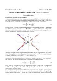
To bring this series in a less complicated form, let us first look at A (2) (t, t0):<br />
� t<br />
t0<br />
dτ1<br />
� τ1<br />
t0<br />
dτ2X(τ1)X(τ2). (1.21)<br />
The range of the integration variables is the triangle in the τ1τ2-plane shown at figure 1.1:<br />
00000000<br />
11111111<br />
0000000<br />
1111111<br />
00000000<br />
11111111<br />
00000000<br />
11111111<br />
00000000<br />
11111111<br />
00000000<br />
11111111<br />
00000000<br />
11111111<br />
00000000<br />
11111111<br />
00 11<br />
00000000<br />
11111111<br />
00 11 01<br />
01<br />
t<br />
t0<br />
τ2<br />
t0<br />
t<br />
t2 = t2<br />
Figure 1.1: Range of integration variables in (1.21)<br />
Using Fubini’s theorem we can interchange the integrations<br />
A (2) =<br />
� t<br />
t0<br />
dτ1<br />
� t<br />
τ1<br />
τ1<br />
dτ2X(τ1)X(τ2). (1.22)<br />
A glance at the opera<strong>to</strong>r ordering in (1.21) and (1.22) shows that it is such that the opera<strong>to</strong>r at<br />
the later time is always on the left. For this, one introduces the causal time ordering opera<strong>to</strong>r Tc,<br />
invented by Dyson. With help of Tc, one can add both equations, leading <strong>to</strong> the result<br />
2A (2) (t, t0) = Tc<br />
� t<br />
t0<br />
dτ1<br />
� t<br />
t0<br />
dτ2X(τ1)X(τ2). (1.23)<br />
We state that this observation holds for the general case of an arbitrary summand in the series<br />
(1.20), i.e.,<br />
A (k) (t, t0) = 1<br />
k! Tc<br />
� t � t<br />
dτ1 · · · dτnX(τ1) · · · X(τn). (1.24)<br />
t0<br />
To prove this assumption, we use an induction argument. Assume the assumption is true for<br />
k = n − 1 and look at the nth summand of the series. Because the assumption is true for k = n − 1,<br />
we can apply it <strong>to</strong> the n − 1 inner integrals:<br />
A (n) (t, t0) =<br />
1<br />
(n − 1)! Tc<br />
� t<br />
t0<br />
dτ1<br />
� τ1<br />
t0<br />
17<br />
t0<br />
� τ1<br />
dτ2 · · ·<br />
t0<br />
dτnX(τ1) · · · X(τn). (1.25)
Chapter 1 · Path Integrals<br />
Now we can do the same calculation as we did for A (2) with the outer integral and one of the inner<br />
ones. Adding all the possibilities of pairing and dividing by n one gets immediately<br />
A (n) (t, t0) = 1<br />
n! Tc<br />
� t<br />
t0<br />
dτ1 · · ·<br />
and that is (1.24) for k = n. So, our assumption is proven by induction.<br />
� t<br />
t0<br />
dτnX(τ1) · · · X(τn), (1.26)<br />
With this little combina<strong>to</strong>rics we can write the series formally as<br />
� � t �<br />
A(t, t0) = Tc exp i dτX(τ) . (1.27)<br />
This is the required formal solution of the equation of motion. For the opera<strong>to</strong>r C(t, t0) one finds<br />
the solution by the same manipulations <strong>to</strong> be:<br />
� � t �<br />
C(t, t0) = Tc exp −i dτY(τ) . (1.28)<br />
1.4 Example: The Free Particle<br />
The most simple example is the free particle. For calculating the time development of quantum<br />
mechanical quantities, we chose the Heisenberg picture defined in terms of the above introduced<br />
time evolution opera<strong>to</strong>rs X = H and Y = 0. We take as an example a free point particle moving in<br />
one-dimensional space. The fundamental algebra is given by the space and the momentum opera<strong>to</strong>r<br />
which fulfil the Heisenberg algebra<br />
1<br />
[x, p] = 1, (1.29)<br />
i<br />
which follows from the rules of canonical quantisation from the Poisson bracket relation in Hamil<strong>to</strong>nian<br />
mechanics or from the fact that the momentum is defined as the genera<strong>to</strong>r of translations in<br />
space.<br />
As said above, in the Heisenberg picture only the opera<strong>to</strong>rs, representing observables, depend on<br />
time, and the states are time independent. To solve the problem of time evolution we can solve the<br />
opera<strong>to</strong>r equations of motion for the fundamental opera<strong>to</strong>rs rather than solving the equation for<br />
the time evolution opera<strong>to</strong>r. The Hamil<strong>to</strong>nian for the free particle is given by<br />
t0<br />
t0<br />
H = p2<br />
, (1.30)<br />
2m<br />
where m is the mass of the particle. The opera<strong>to</strong>r equations of motion can be obtained from the<br />
general rule (1.14) with X = H:<br />
dp<br />
dt<br />
1<br />
dx 1<br />
= [p, H] = 0, =<br />
i dt i<br />
p<br />
[x, H] = . (1.31)<br />
m<br />
This looks like the equation for the classical case, but it is an opera<strong>to</strong>r equation. But in our case<br />
that doesn’t affect the solution which is given in the same way as the classical one by<br />
p(t) = p(0) = const, x(t) = x(0) + p<br />
t. (1.32)<br />
m<br />
18
1.4 · Example: The Free Particle<br />
Here, without loss of generality, we have set t0=0.<br />
Now let us look on the time evolution of the wave function given as the matrix elements of the<br />
state ket and a complete set of orthonormal eigenvec<strong>to</strong>rs of observables. We emphasise that the<br />
time evolution of such a wave function is up <strong>to</strong> a phase independent of the choice of the picture.<br />
So we may use any picture we like <strong>to</strong> get the answer. Here, we use the Heisenberg picture, where<br />
the state ket is time independent. The whole time dependence comes from the eigenvec<strong>to</strong>rs of the<br />
observables. As a first example we take the momentum eigenvec<strong>to</strong>rs and calculate the wave function<br />
in the momentum representation. From (1.31) we get up <strong>to</strong> a phase:<br />
�<br />
|p, t〉 = exp(iHt) |p, 0〉 = exp i p2<br />
2m t<br />
�<br />
|p, 0〉 , (1.33)<br />
and the time evolution of the wave function is simply<br />
�<br />
ψ(p, t) = 〈p, t | ψ 〉 = exp −i p2<br />
2m t<br />
�<br />
ψ(p, 0). (1.34)<br />
This can be described by the operation of an integral opera<strong>to</strong>r in the form<br />
�<br />
�<br />
ψ(p, t) =<br />
From (1.32) one finds<br />
dp ′ � p, t � � p ′ , 0 �<br />
� �� �<br />
U(t,p;0,p ′ � �<br />
′<br />
p , 0 � ψ<br />
)<br />
� =<br />
dp ′ U(t, p; 0, p ′ )ψ(p ′ , 0). (1.35)<br />
U(t, p, 0, p ′ �<br />
) = exp −i p2<br />
2m t<br />
�<br />
δ(p − p ′ ). (1.36)<br />
It should be kept in mind from this example that the time evolution kernels or propaga<strong>to</strong>rs which<br />
define the time development of wave functions are in general distributions rather than functions.<br />
The next task, we like <strong>to</strong> solve, is the propaga<strong>to</strong>r in the configuration-space representation of the<br />
wave function. We will give two approaches: First we start anew and calculate the space eigenvec<strong>to</strong>rs<br />
from the solution of the opera<strong>to</strong>r equations of motion (1.32). We have by definition:<br />
�<br />
x(t) |x, t〉 = x(0) + p(0)<br />
m t<br />
�<br />
|x, t〉 = x |x, t〉 . (1.37)<br />
Multiplying this with 〈x ′ , 0| we find by using the representation of the momentum opera<strong>to</strong>r in space<br />
representation p = 1/i∂x:<br />
which is solved in a straight forward way:<br />
(x ′ − x) � x ′ , 0 � � x, t � = it � �<br />
′<br />
∂x ′ x , 0 � x, t<br />
m �<br />
U(t, x; 0, x ′ ) ∗ = � x ′ , 0 � � x, t � = N exp<br />
(1.38)<br />
�<br />
−i m<br />
2t (x′ − x) 2�<br />
. (1.39)<br />
Now we have <strong>to</strong> find the complex normalisation fac<strong>to</strong>r N. It is given by the initial condition<br />
U(0, x; 0, x ′ ) = δ(x − x ′ ) (1.40)<br />
19
Chapter 1 · Path Integrals<br />
which also determines its phase and the fact that U is the matrix element of a unitary opera<strong>to</strong>r:<br />
�<br />
dx ′ U(t, x1; 0, x ′ )U ∗ (t, x2; 0, x ′ ) = δ(x1 − x2). (1.41)<br />
Using (1.39), this integral gives<br />
�<br />
dx ′ U(t, x1; 0, x ′ )U ∗ (t, x2; 0, x ′ 2 2πt<br />
) = |N|<br />
m δ(x1 − x2),<br />
�<br />
m<br />
→ N = exp(iα).<br />
2πt<br />
(1.42)<br />
To determine the phase, we use (1.40). It is most simple <strong>to</strong> fold U with an arbitrary L2 function,<br />
for which we choose the Gaussian exp(−ax2 ):<br />
�<br />
dx ′ U(t, x; 0, x ′ ) exp(−ax ′2 �<br />
1<br />
) =<br />
2at/m − i exp<br />
�<br />
− amx2<br />
�<br />
+ iα . (1.43)<br />
m + 2iat<br />
The square root is unders<strong>to</strong>od as its principle value, i.e., for t > 0 it has a positive imaginary part.<br />
Now taking the limit t → 0+ it becomes exp(+iπ/4) and thus we must have α = −π/4, yielding the<br />
final result or the propaga<strong>to</strong>r:<br />
U(t, x; 0, x ′ �<br />
m<br />
) =<br />
2πit exp<br />
�<br />
im<br />
2t (x − x′ ) 2<br />
�<br />
. (1.44)<br />
An alternative possibility <strong>to</strong> get this result is <strong>to</strong> use the momentum space result and transform it<br />
<strong>to</strong> space representation. We leave this nice calculation as an exercise for the reader. For help we<br />
give the hint that again one has <strong>to</strong> regularise the distribution <strong>to</strong> give the resulting Fourier integral<br />
a proper meaning.<br />
1.5 The Feynman-Kac Formula<br />
Now we are at the right stage for deriving the path integral formalism of quantum mechanics. In<br />
these lectures we shall often switch between opera<strong>to</strong>r formalism and path integral formalism. We<br />
shall see that both approaches <strong>to</strong> quantum theory have their own advantages and disadvantages.<br />
The opera<strong>to</strong>r formalism is quite nice <strong>to</strong> see the unitarity of the time evolution. On the other hand<br />
the canonical quantisation procedure needs the Hamil<strong>to</strong>nian formulation of classical mechanics <strong>to</strong><br />
define Poisson brackets which can be mapped <strong>to</strong> commuta<strong>to</strong>rs in the quantum case. This is very<br />
inconvenient for the relativistic case because we have <strong>to</strong> treat the time variable in a different way<br />
than the space variables. So the canonical formalism hides relativistic invariance leading <strong>to</strong> non<br />
covariant rules at intermediate steps. <strong>Relativistic</strong> invariance will be evident at the very end of the<br />
calculation.<br />
Additional <strong>to</strong> this facts which are rather formal we shall like <strong>to</strong> discuss gauge theories like electrodynamics<br />
or the standard model. The quantisation of theories of that kind is not so simple <strong>to</strong> formulate<br />
in the opera<strong>to</strong>r formalism but the path integral is rather nice <strong>to</strong> handle. It is also convenient <strong>to</strong> use<br />
functional methods <strong>to</strong> derive formal properties of quantum field theories as well as such practical<br />
important <strong>to</strong>pics like Feynman graphs for calculating scattering amplitudes perturbatively.<br />
20
1.5 · The Feynman-Kac Formula<br />
In this section we shall take a closer look on path integrals applied <strong>to</strong> nonrelativistic quantum<br />
mechanics.<br />
For sake of simplicity we look again on a particle in one configuration space dimension moving in<br />
a given potential V . Again we want <strong>to</strong> calculate the time evolution kernel U(t ′ , x ′ ; t, x) which was<br />
given in the previous chapter in terms of the Heisenberg picture space coordinate eigenstates:<br />
� x ′ , t ′ � � x, t � = � x ′ , 0 � �exp[−iH(t ′ − t)] � � x, 0 �<br />
(1.45)<br />
where we have used the solution of the equation of motion for Hamil<strong>to</strong>nian which is explicitly time<br />
independent, i.e. in the Heisenberg picture it is a function of the fundamental opera<strong>to</strong>rs, here taken<br />
as x and p alone. We consider at the moment the most simple case which in fact covers a wide<br />
range of application in the case of nonrelativistic quantum mechanics:<br />
H = p2<br />
+ V (x). (1.46)<br />
2m<br />
We will take in<strong>to</strong> account more general cases later. The idea behind our derivation of the path<br />
integral formula is quite simple. Because we know the time evolution explicitly for very small time<br />
intervals, namely it is given by the Hamil<strong>to</strong>nian, it seems <strong>to</strong> be sensible <strong>to</strong> divide the time interval<br />
(t,t’) in N equal pieces (in the following called time slices) of length ∆t = (t ′ − t)/N. Since the<br />
Hamil<strong>to</strong>nian is not explicitly time dependent which means in the Heisenberg picture that it is a<br />
constant of motion (see eq. (1.14) and keep in mind that in the Heisenberg picture we have by<br />
definition X = H) we can write the time evolution opera<strong>to</strong>r in the “time sliced” form<br />
exp[−iH(t ′ − t)] = exp(−iH∆t) exp(−iH∆t) . . . exp(−iH∆t) . (1.47)<br />
� �� �<br />
N times<br />
Now there is the problem that x and p are not commuting. But one can show easily, that there<br />
holds the following formula<br />
by expanding both sides of the equation in orders of λ.<br />
exp[λ(A + B)] = exp λA exp λB + O(λ 2 ) (1.48)<br />
From this we can hope that with N → ∞ the error made by splitting the time evolution opera<strong>to</strong>r<br />
in the form<br />
�<br />
exp(−i∆tH) = exp −i∆t p2<br />
�<br />
exp[−i∆tV (x)] + O(∆t<br />
2m<br />
2 ) (1.49)<br />
and neglecting the terms of order ∆t 2 becomes negligible. Now splitting the time evolution opera<strong>to</strong>r<br />
in this way we may put a unity opera<strong>to</strong>r in between which is written as the spectral representation<br />
21
� dx |x〉 〈x| or � dp |p〉 〈p| in the following way:<br />
U(t ′ , x ′ ; t, x) =<br />
�<br />
Chapter 1 · Path Integrals<br />
dp1 . . . dpNdx2 . . . dxN ×<br />
�<br />
× x ′<br />
�<br />
�<br />
�<br />
�exp �<br />
−i∆t p2<br />
�� �<br />
���<br />
pN 〈pN |exp[−i∆tV (x)]| xN〉 ×<br />
2m<br />
� �<br />
�<br />
× xN<br />
�<br />
�exp �<br />
−i∆t p2<br />
�� �<br />
���<br />
pN−1 〈pN−1 |exp[−i∆tV (x)]| xN−1〉 ×<br />
2m<br />
× · · · ×<br />
� �<br />
�<br />
× x2 �<br />
�exp �<br />
−i∆t p2<br />
�� �<br />
���<br />
p1 〈p1 |exp(−i∆tV )| x〉 , (1.50)<br />
2m<br />
where, in the latter sum, we have set x1 = x ′ and xN+1 = x. Now the two different sorts of matrix<br />
elements arising in this expression are trivially calculated <strong>to</strong> be<br />
� �<br />
�<br />
xk+1<br />
�<br />
�exp �<br />
−i∆t p2<br />
�� � �<br />
���<br />
pk = exp −i∆t<br />
2m<br />
p2 �<br />
k exp(ipkxk+1)<br />
√ (1.51)<br />
2m 2π<br />
〈pk |exp(−i∆tV )| xk〉 = exp[−i∆tV (xk)] exp(−ixkpk)<br />
√ , (1.52)<br />
2π<br />
where we have used the correctly “normalised” momentum eigenstate in the configuration-qspace<br />
representation:<br />
〈x | p〉 = exp(ixp)<br />
√ 2π . (1.53)<br />
Putting all this <strong>to</strong>gether we obtain the time sliced form of the path integral formula which is named<br />
after its inven<strong>to</strong>rs Feynman-Kac formula:<br />
U(t ′ , x ′ �<br />
; t, x) = lim dp1 . . . dpNdx2 . . . dxN−1 ×<br />
N→∞<br />
� � �<br />
N<br />
N�<br />
�<br />
1<br />
p2 � N�<br />
�<br />
k<br />
× exp −i∆t + V (xk) + i pk(xk+1 − xk) , (1.54)<br />
2π<br />
2m<br />
k=1<br />
Now we interpret this result in another way than we have obtained it. The pairs (xk, pk) <strong>to</strong>gether<br />
can be seen as a discrete approximation of a path in phase space parametrised by the time. The<br />
mentioned points are defined <strong>to</strong> be (x(tk), p(tk)) on the path. Then the sum in the argument of the<br />
exponential function is an approximation for the following integral along the given path:<br />
� t ′<br />
t<br />
k=1<br />
�<br />
dt −H(x, p) + p dx<br />
�<br />
. (1.55)<br />
dt<br />
Now we should remember that we have fixed the endpoints of the path in configuration space <strong>to</strong><br />
be x(t) = x and x(t ′ ) = x ′ . So we have the following interpretation of the Feynman-Kac formula<br />
after taking the limit N → ∞: The time evolution kernel U(x ′ , t ′ ; x, t) is the sum of the functional<br />
exp(iS[x, p]) over all paths beginning at time t at the point x ending at the point x ′ at time t ′ .<br />
22
1.5 · The Feynman-Kac Formula<br />
For the momenta there is no boundary condition at all. This is quite o.k., because we have no<br />
restriction on the momenta. Because of the uncertainty relation it does not make any sense <strong>to</strong><br />
have such conditions on both x and p at the same time! The action S is here seen as a functional<br />
depending on the paths in phase space which fulfil this boundary conditions:<br />
S[x, p] =<br />
� t ′<br />
t<br />
�<br />
dt p dx<br />
�<br />
− H(x, p) . (1.56)<br />
dt<br />
We conclude that the formula (1.54) may be taken as the definition of the continuum limit of the<br />
path integral, written symbolically as<br />
U(t ′ , x ′ � (t ′ ,x ′ )<br />
; t, x) =<br />
(t,x)<br />
DpDx exp {iS[x, p]} . (1.57)<br />
The physical interpretation is now quite clear: The probability that the particle known <strong>to</strong> be at<br />
time t exactly at the point x is at time t ′ exactly at the point x ′ is given with help of the time<br />
evolution kernel in space representation as |U(t ′ , x ′ ; t, x)| 2 and the amplitude is given as the coherent<br />
sum over all paths with the correct boundary conditions. All paths in phase space contribute <strong>to</strong><br />
this sum. Because the boundary space points x and x ′ are exactly fixed at the given times t and<br />
t ′ respectively it is quantum mechanically impossible <strong>to</strong> know anything about the momenta at this<br />
times. Because of that typical quantum mechanical feature there are no boundary conditions for<br />
the momenta in the path integral!<br />
Now let us come back <strong>to</strong> the discretised version (1.54) of the path integral. Since the Hamil<strong>to</strong>nian<br />
is quadratic in p the same holds for the p-dependence of the exponential in this formula. So the<br />
p-integrals can be calculated exactly. As seen above we have <strong>to</strong> regularise it by giving the time<br />
interval ∆t a negative imaginary part which is <strong>to</strong> be tent <strong>to</strong> zero after the calculation. For one of<br />
the momentum integrals this now familiar procedure gives the result<br />
�<br />
Ik =<br />
�<br />
dpk exp −i∆t p2 k<br />
2m + ipk(xk<br />
�<br />
− xk−1) =<br />
� 2πm<br />
i∆t exp<br />
� im(xk − xx−1) 2<br />
2∆t<br />
�<br />
. (1.58)<br />
Inserting this result in eq. (1.54) we find the configuration space version of the path integral formula:<br />
U(t ′ , x ′ �<br />
; t, x) = lim<br />
N→∞<br />
dx1 . . . dxN<br />
� �<br />
N<br />
m<br />
exp i<br />
2πi∆t<br />
N�<br />
�<br />
m(xk − xk−1) 2<br />
k=1<br />
2∆t<br />
As above we can see that this is the discretised version of the path integral<br />
U(t ′ , x ′ � t ′ ,x ′<br />
; t, x) =<br />
t,x<br />
�<br />
− V (xi)∆t<br />
�<br />
. (1.59)<br />
D ′ x exp{iS[x]}, (1.60)<br />
where we now obtained S[x] = � t ′<br />
t dtL, i.e. the action as a functional of the path in configuration<br />
space. The prime on the path integral measure is <strong>to</strong> remember that there are the square root fac<strong>to</strong>rs<br />
in (1.59).<br />
23
Chapter 1 · Path Integrals<br />
With that manipulation we have obtained an important feature of the path integral: It is a description<br />
which works with the Lagrangian version of classical physics rather than with the Hamil<strong>to</strong>nian<br />
form. This is especially convenient for relativistic physics, because then the Hamil<strong>to</strong>nian formalism<br />
is not manifestly covariant.<br />
It was Feynman who invented the path integrals in 1942 in his Ph.D. thesis. Later on he could use it<br />
as a <strong>to</strong>ol for finding the famous Feynman graphs for perturbative QED which we shall derive later in<br />
our lectures. That Feynman graphs give a very suggestive picture of the scattering processes of the<br />
particles due <strong>to</strong> electromagnetic interaction among them. In the early days of quantum field theory<br />
Schwinger and Feynman wondered why they obtained the same results in QED. Schwinger was using<br />
his very complicated formal field opera<strong>to</strong>r techniques and Feynman his more or less handwaving<br />
graphical arguments derived from his intuitive space-time picture. Later on Dyson derived the<br />
Feynman rules formally from the canonical quantisation of classical electrodynamics and that was<br />
the standard way getting the rules for calculating scattering cross sections etc. With the advent<br />
of non-Abelian gauge theories in the late fifties and their great breakthrough in the early seventies<br />
(electro weak theory, renormalisability of gauge theories) this has changed completely: Nowadays<br />
the path integral formalism is the standard way <strong>to</strong> obtain the content of the theory for all physicists<br />
who are interested in theoretical many body quantum physics.<br />
After this little his<strong>to</strong>rical sideway let us come back <strong>to</strong> the path integrals themselves. Now it is<br />
time <strong>to</strong> get some feeling for it by applying it <strong>to</strong> the most simple nontrivial example which can be<br />
calculated in a closed form: The harmonic oscilla<strong>to</strong>r.<br />
1.6 The Path Integral for the Harmonic Oscilla<strong>to</strong>r<br />
The harmonic oscilla<strong>to</strong>r is defined by the Lagrangian<br />
L = m<br />
2 ˙x2 − mω2<br />
2 x2 . (1.61)<br />
The corresponding Hamil<strong>to</strong>nian is quadratic not only in p but also in x. This is the reason, why<br />
we can calculate the path integral exactly in this case. We will use the discretised version (1.59) of<br />
the configuration space path integral.<br />
The biggest problem is the handling of the boundary conditions of the path. Fortunately this<br />
problem can be solved by parameterising the path relative <strong>to</strong> the classical one defined as that path<br />
which extremises the action S[x]:<br />
δS[x]<br />
δx<br />
�<br />
�<br />
�<br />
� x=xcl<br />
= 0 with x(t) = x, x(t ′ ) = x ′ . (1.62)<br />
Since the action is quadratic it can be expanded around the classical path and the series will end<br />
with the summand of second order in y = x − xcl:<br />
S[y + xcl] = S[xcl] + 1<br />
�<br />
δ<br />
2<br />
2 � �<br />
S �<br />
� y1y2 , (1.63)<br />
δx1δx2<br />
24<br />
� x=xcl<br />
12
1.6 · The Path Integral for the Harmonic Oscilla<strong>to</strong>r<br />
where the bracket is a shorthand notation with the following meaning<br />
� t ′<br />
〈f12...n〉<br />
12...n =<br />
t<br />
The term linear in y does not contribute because of (1.62).<br />
dt1dt2 . . . dtnf(t1, t2, . . . , tn). (1.64)<br />
Since we have <strong>to</strong> sum over all paths x with the boundary conditions fulfilled by the classical path<br />
this can be expressed as sum over all paths y with the easier <strong>to</strong> handle boundary conditions y(t) =<br />
y(t ′ ) = 0. Formally this is done by substitution y = x−xcl in<strong>to</strong> the path integral. Thinking in terms<br />
of the discretised version of the path integral one immediately sees that the path integral measure<br />
is invariant under time dependent translations of x, i.e. D ′ x = D ′ y. So we get the important result<br />
U(t ′ , x ′ � (t ′ ,0)<br />
; t, x) = exp{iS[xcl]} D<br />
(t,0)<br />
′ � � ��<br />
i δS[xcl]<br />
y exp<br />
y1y2<br />
2 δx1δx2<br />
t<br />
(1.65)<br />
As the first step we calculate the action along the classical path. We have <strong>to</strong> calculate the functional<br />
derivative of S with fixed boundary conditions.<br />
� t ′ � �<br />
∂L ∂L<br />
δS = dt δx + δ ˙x . (1.66)<br />
∂x ∂ ˙x<br />
By integration by parts with taking in<strong>to</strong> account the boundary conditions δx(t) = δx(t ′ ) = 0 we<br />
obtain<br />
� t ′ � �<br />
∂L d ∂L<br />
δS = dt − δx.<br />
∂x dt ∂ ˙x<br />
(1.67)<br />
t<br />
So the equations of motion defining the classical path are given by the Euler Lagrange equations<br />
with the Lagrangian L:<br />
0 = δS<br />
� � �<br />
�<br />
�<br />
∂L d ∂L<br />
δx � = − . (1.68)<br />
∂x dt ∂ ˙x<br />
x=xcl<br />
x=xcl<br />
It is clear that we get the equation of the classical motion of the harmonic oscilla<strong>to</strong>r. The equation<br />
with the correct boundary conditions defined in (1.62) is simple <strong>to</strong> solve:<br />
xcl(τ) = x cos[ω(τ − t)] + x′ − x cos[ω(t ′ − t)]<br />
sin[ω(t ′ − t)]<br />
From this result the action along the classical path is given by<br />
sin[ω(τ − t)]. (1.69)<br />
S[xcl] = mω{(x2 + x ′2<br />
) cos[ω(t ′ − t)] − 2xx ′ }<br />
2 sin[ω(t ′ . (1.70)<br />
− t)]<br />
To finish the calculation now we are left with the path integral in (1.65) with the homogeneous<br />
boundary conditions. This has <strong>to</strong> be calculated in the discretised version. We call the path integral<br />
the amplitude A:<br />
�<br />
mN<br />
A = lim<br />
N→∞ 2πi(t ′ �N/2 �<br />
− t)<br />
dy1 . . . dyN−1 exp<br />
25<br />
�<br />
i<br />
N�<br />
�<br />
m(yk − yk−1) 2<br />
k=1<br />
2∆t<br />
− m2<br />
2 ω2y 2 k∆t �� (1.71)
Chapter 1 · Path Integrals<br />
Since y0 = yN = 0 the argument of the exponential function can be written as<br />
N�<br />
�<br />
m(yk − yk−1) 2<br />
k=1<br />
2∆t<br />
where �y is the column vec<strong>to</strong>r (y1, y2, . . . , yN−1) and<br />
⎛<br />
⎜<br />
MN = ⎜<br />
⎝<br />
C −1 0 0 0 · · ·<br />
−1 C −1 0 0 · · ·<br />
0 −1 C −1 0 · · ·<br />
.<br />
.<br />
.<br />
− m2<br />
2 ω2y 2 k∆t �<br />
= m<br />
2∆t �yt MN�y, (1.72)<br />
.<br />
.<br />
.<br />
⎞<br />
⎟<br />
⎠ with C = 2 − ω2∆t 2<br />
(1.73)<br />
Now we calculate the k-dimensional Gaussian integral with a symmetric positive definite matrix M.<br />
Since such matrices can be diagonalised by an orthogonal transformation we get<br />
�<br />
d k y exp(−y t My) =<br />
k�<br />
�<br />
j=1<br />
dxj exp(−λjx 2 j), (1.74)<br />
where we have substituted z = Ox. The λj are the eigenvalues of the matrix M. So the problem<br />
reduces <strong>to</strong> the product of single Gaussian integrals:<br />
�<br />
d k y exp(−y t My) =<br />
� π k<br />
� k<br />
j=1 λj<br />
�<br />
πk = . (1.75)<br />
detM<br />
So after giving ∆t a negative imaginary value and analytic continuation back <strong>to</strong> the real value<br />
(t ′ − t)/N (determinants are analytic functions of the matrix elements) our problem <strong>to</strong> calculate<br />
(1.71) is reduced <strong>to</strong> calculate the determinant of MN. That will be done as an exercise because the<br />
calculation is lengthy and tedious. The result after taking the continuum limit N → ∞ gives the<br />
result for the amplitude:<br />
�<br />
mω<br />
A =<br />
2πi sin[ω(t ′ . (1.76)<br />
− t)]<br />
Thus the final result is<br />
U[x ′ , t ′ �<br />
mω<br />
; x, t] =<br />
2πi sin[ω(t ′ − t)] exp<br />
�<br />
imω{(x2 + x ′2<br />
) cos[ω(t ′ − t)] − 2xx ′ }<br />
2 sin[ω(t ′ �<br />
, (1.77)<br />
− t)]<br />
where we have put <strong>to</strong>gether (1.65), (1.66) and (1.76).<br />
Exercise<br />
Calculate the determinant of MN, put it in<strong>to</strong> (1.71-1.72) <strong>to</strong> prove (1.76)! Hint: It is useful <strong>to</strong> set<br />
C = 2 cos φ in (1.73).<br />
26
1.7 · Some Rules for Path Integrals<br />
1.7 Some Rules for Path Integrals<br />
Now that we have calculated a closed solvable example, we can derive some general properties of<br />
path integrals. The first one we get by writing down the composition rule (1.11), which is valid for<br />
our time evolution kernel <strong>to</strong>o, in terms of path integrals. For t1 < t2 < t3 we have<br />
� (t3,x3)<br />
(t1,x1)<br />
D ′ �<br />
x exp{iS[x]} =<br />
dx2<br />
� (t2,x2)<br />
(t1,x1)<br />
D ′ x exp{iS[x]}<br />
� (t3,x3)<br />
(t2,x2)<br />
D ′ x exp{iS[x]}. (1.78)<br />
This formula can be proved with help of the discretised version of the path integral formula. That<br />
easy task is left as an exercise for the reader.<br />
We can give a more intuitive explanation of this composition rule. The left hand side of the equation<br />
gives the sum of the functional exp{iS[x]} over all paths of the particle with the boundary conditions<br />
x(t1) = x1 <strong>to</strong> x(t3) = x3. On the right hand side the both path integrals are the sum of the same<br />
functional over all paths with the same boundary conditions but with the constraint x(t2) = x2 for<br />
a time in the interval (t1, t3), i.e. over all paths with the particle at a given place x2 at time t2.<br />
Now this restriction is compensated by the single integral over all intermediate positions x2. So the<br />
left and the right hand side of the equation are indeed the same!<br />
Now there is no problem <strong>to</strong> obtain a little bit more complicated quantities in terms of path integrals.<br />
As an example which will become crucial in the quantum field case we shall calculate the expectation<br />
value of a product of Heisenberg configuration space opera<strong>to</strong>rs at different times. If this times are<br />
ordered in the sense of the causal time ordering opera<strong>to</strong>r introduced after eq. (1.32), that means<br />
that the time values of the opera<strong>to</strong>rs increase from the right <strong>to</strong> the left, there is no problem. Using<br />
the unit opera<strong>to</strong>r given in terms of x-eigenstates at the given times and applying the composition<br />
rule of path integrals we obtain the following rule<br />
� x ′ , t ′ � � Tcx(t1)x(t2) . . . x(tk) � � x, t � =<br />
� (t ′ ,x ′ )<br />
(t,x)<br />
1.8 The Schrödinger Wave Equation<br />
D ′ xx(t1)x(t2) . . . x(tk) exp{iS[x]}. (1.79)<br />
In this section we want <strong>to</strong> derive Schrödinger’s wave equation for the kernel of time evolution. The<br />
main idea is <strong>to</strong> show, how <strong>to</strong> find such equations from the path integral. We start again with the<br />
Feynman-Kac formula for the time evolution kernel for t ′ > t:<br />
U(t ′ , x ′ � (t ′ ,x ′ )<br />
; t, x) =<br />
(t,x)<br />
D ′ x exp{iS[x]}. (1.80)<br />
Now we want <strong>to</strong> calculate the time derivative of this expression with respect <strong>to</strong> t ′ . So let ɛ be a<br />
little increment of t ′ . Now by the composition rule one has<br />
�<br />
U(t ′ + ɛ, x ′ ; t, x) =<br />
dξU(t ′ + ɛ, x ′ ; t ′ , ξ)U(t ′ , ξ; x, t). (1.81)<br />
27
Chapter 1 · Path Integrals<br />
Now we try <strong>to</strong> find the expansion with respect <strong>to</strong> ɛ. Since it can be thought <strong>to</strong> be very small<br />
compared <strong>to</strong> the typical time scale of the problem we can approximate the first kernel on the right<br />
hand side by a path integral with just one time slice namely the interval (t ′ , t ′ + ɛ). So we get<br />
U(t ′ , x ′ ; t, x) =<br />
�<br />
�<br />
m<br />
dξ<br />
2πiɛ exp<br />
�<br />
i m(x′ − ξ) 2 �<br />
[1 − iɛV (x<br />
2ɛ<br />
′ ) + O(ɛ 2 )]U(t ′ , ξ; t, x). (1.82)<br />
Since we like <strong>to</strong> calculate this expression for ɛ → 0 the exponential is oscillating rapidly except for<br />
values ξ ≈ x ′ . In a mathematically more correct treatment we could have continued the time <strong>to</strong> be<br />
imaginary instead of regularising the path integral by only a little negative imaginary part. If we had<br />
done so the exponential is not oscillating but damped. From the imaginary time formalism we obtain<br />
the correct time evolution kernel by analytic continuation. So we see that the main contribution<br />
of the ξ-integral comes from ξ ≈ x ′ . By changing the variable of integration <strong>to</strong> δ = x ′ − ξ and<br />
expanding U(t ′ , ξ; t, x) around δ we obtain<br />
U(t ′ + ɛ, x ′ � � � �<br />
m imδ2 ; t, x) = dδ<br />
[1 − ɛV (x ′ ) + O(ɛ 2 )] ×<br />
×<br />
� ∞�<br />
k=0<br />
2πiɛ exp<br />
�<br />
∂<br />
∂x ′<br />
�k 2ɛ<br />
U(t ′ , x ′ ; t, x) (−δ)k<br />
k!<br />
�<br />
. (1.83)<br />
Now interchanging integration and summation of the series we need integrals of a Gaussian multiplied<br />
by any potence of δ. This integrals can be obtained by defining a generating function:<br />
f(Λ) =<br />
� �<br />
m<br />
2πiɛ exp<br />
� �<br />
imδ2 + Λδ . (1.84)<br />
2ɛ<br />
After the usual regularisation by an negative imaginary part for ɛ we can calculate this integral and<br />
from this we find<br />
�<br />
Ik =<br />
�<br />
m<br />
dδ<br />
2πiɛ δk � �<br />
imδ2 exp =<br />
2ɛ<br />
dkf(Λ) dΛk �<br />
�<br />
� . (1.85)<br />
For ɛ → 0 we need only the following identities<br />
Inserting this in<strong>to</strong> (1.83) we get<br />
� Λ=0<br />
I0 = 1, I1 = 0, I2 = iɛ<br />
m , I2n = O(ɛ n ), I2n+1 = 0 for n ∈ N. (1.86)<br />
U(t ′ + ɛ, x ′ ; t, x) = [1 − iɛV (x ′ ) + O(ɛ 2 )]<br />
Subtracting U(t ′ , x ′ ; t, x) and letting ɛ → 0 we obtain the important result<br />
i∂t ′U(t′ , x ′ �<br />
; t, x) = − 1<br />
2m ∂2 x ′ + V (x′ �<br />
)<br />
�<br />
1 + iɛ<br />
2m ∂2 x ′<br />
�<br />
U(t ′ , x ′ ; t, x). (1.87)<br />
U(t ′ , x ′ ; t, x) for t ′ > t. (1.88)<br />
This is the Schrödinger equation, since the differential opera<strong>to</strong>r on the right hand side is the Hamil<strong>to</strong>nian<br />
expressed in terms of configuration space representation. The initial condition for the kernel,<br />
necessary <strong>to</strong> make the solution of the Schrödinger equation unique, is of course<br />
U(t + 0, x ′ ; t, x) = δ(x ′ − x). (1.89)<br />
28
1.9 · Potential Scattering<br />
This is the first time we see that the time evolution kernel is nothing but the Green’s function of<br />
the Schrödinger equation. We will get a deeper insight in this relation by looking on an important<br />
physical application of all the developed formalism, namely the perturbative treatment of potential<br />
scattering with help of path integrals.<br />
1.9 Potential Scattering<br />
Potential scattering is an example where the path integral formalism is very intuitive. The setup<br />
of a scattering experiment can described in the following idealised way: The physicist prepares a<br />
beam of particles with a definite momentum �pi far away from the target where it will be scattered.<br />
After the scattering process the physicist will use detec<strong>to</strong>rs, again far away from the scatterer, <strong>to</strong><br />
find the rate of scattered particles as a function of their momentum �pf .<br />
Now let us describe this from a little bit more mathematical point of view: Since we want <strong>to</strong> look<br />
on the most simple situation now, we give the scatterer in terms of a external potential. So we<br />
have only one particle scattered by this external potential. This is approximately realized by the<br />
scattering of a particle on another particle with a much greater mass (e.g. scattering of an electron<br />
at a heavy nucleus). This potential should have only a finite range, i.e., V (�x) should be very small<br />
for |�x| > R, where R is a typical range scale of the potential. So the particles prepared before the<br />
scattering and registered after the scattering, far away from �x = 0, that means now |�x| > R, can be<br />
treated as quasi free particles. This is what is widely known as an asymp<strong>to</strong>tic free state.<br />
Now let us analyse this situation with help of quantum mechanics. What we like <strong>to</strong> calculate is<br />
the transition rate of particles which are prepared at an initial time t0 → −∞ as asymp<strong>to</strong>tic free<br />
particles of definite momentum �pi <strong>to</strong> a given asymp<strong>to</strong>tic free state of definite momentum �pf at a<br />
time tf . In the Heisenberg picture this is simply written as<br />
Sfi = lim<br />
ti→−∞,tf →∞ 〈tf , �pf | �pi, ti 〉 . (1.90)<br />
This defines the scattering matrix, shortly called the S-Matrix, as the transition rate from a given<br />
initial asymp<strong>to</strong>tic free state (in our case of definite momentum) <strong>to</strong> a given final asymp<strong>to</strong>tic free<br />
state (in our case also of definite momentum).<br />
It can be seen as the main application of vacuum quantum field theory <strong>to</strong> calculate the S-Matrix<br />
for this and much more complicated processes. We will give a description of scattering from the<br />
quantum field theory point of view later. We will see that in the case of nonrelativistic potential<br />
scattering the both approaches are equivalent. But for example the scattering of two identical<br />
particles is much easier <strong>to</strong> get from the field theoretic point of view than from our space-time<br />
point of view because the space of two identical particles becomes much more complicated than one<br />
should expect from classical physics. We come back <strong>to</strong> this in the next section when we show a very<br />
convincing argument made by Cecile Morette-de Witt about the fact that there can only be bosons<br />
and fermions in a configuration space with three or more dimensions. But let us come now back <strong>to</strong><br />
our potential scattering problem of one particle!<br />
The whole sections before we always calculated the transition amplitudes, i.e. the time evolution<br />
kernel, dependent on space and time variables. Now of course we can look at the scattering process<br />
29
Chapter 1 · Path Integrals<br />
in configuration space <strong>to</strong>o, and we can introduce the time evolution kernel simply by setting some<br />
identity opera<strong>to</strong>rs between the momentum eigenvec<strong>to</strong>rs in (1.90):<br />
�<br />
Sfi = lim<br />
ti→−∞,tf →∞<br />
d 3 �x1d 3 �x2 〈tf , �pf | tf , �x1 〉<br />
� �� �<br />
ϕ∗ 〈tf , �x1 | ti, �x2 〉 〈ti, �x2 | ti, �pi 〉 .<br />
� �� � � �� �<br />
(1.91)<br />
(tf ,�x1)<br />
�p f<br />
U(t1,�x1;tx,�x2) ϕ�pf (ti,�x2)<br />
So we can write the S-Matrix in the form<br />
�<br />
Sfi = lim<br />
d 3 �x1d 3 �x2ϕ ∗ �pf (tf , �x1)U(tf , �x1; ti, �x2)ϕ�pi (ti, �x2), (1.92)<br />
where lim is meant <strong>to</strong> remember <strong>to</strong> take the limit ti → −∞, tf → ∞ at the very end of the<br />
calculation. Herein the wave functions ϕ�p have <strong>to</strong> be taken as the solution of the time dependent<br />
(!) Schrödinger equation for a free particle with definite momentum �p:<br />
�<br />
1<br />
ϕ�p(t, �x) = exp −i<br />
(2π) (3/2) �p2<br />
�<br />
t + i�p�x .<br />
2m<br />
(1.93)<br />
So again the main task is solved if we find a solution for the time evolution kernel or an approximation<br />
appropriate for our situation. In the most cases one has <strong>to</strong> do it in the former sense because it is<br />
impossible <strong>to</strong> find an analytical solution for the kernel. The best method one can use is <strong>to</strong> solve<br />
the Schrödinger equation for the kernel. But here we like <strong>to</strong> give a derivation of the approximation<br />
series known as the Born series with help of the path integral. This has the great advantage <strong>to</strong><br />
give a very intuitive picture of scattering in terms of processes in space-time.<br />
For this purpose we assume now that the potential is small in the sense of a small coupling constant<br />
as is the case, for instance, for electromagnetic forces were the coupling constant is of order of<br />
Sommerfeld’s fine structure constant α = e 2 /(�c) ≈ 1/137. In this case it is sensible <strong>to</strong> expand the<br />
time evolution kernel in powers of the potential.<br />
Our starting point is again the Feynman-Kac formula for the time evolution kernel<br />
U(tf , �x1; ti, �x2) =<br />
� (tf ,�x2)<br />
(ti,�x1)<br />
D ′3 �x exp{iS[�x]}, (1.94)<br />
which is a straight forward generalisation from the one dimensional case, treated so far, <strong>to</strong> the case<br />
of three dimensional configuration space.<br />
Now we have<br />
S[x] =<br />
� tf<br />
ti<br />
[L0(�x, d�x<br />
d�x<br />
) − V (x)]dt with L0(�x,<br />
dt dt ) = S0[x] + SI[x] = m<br />
2<br />
� �2 dx<br />
. (1.95)<br />
dt<br />
Here S0[x] is the action functional of free particles and SI[x] the interaction part of the full action<br />
of the problem. Now we expand the integrand of the path integral in powers of SI:<br />
U(tf , �xf ; ti, �xi) =<br />
×<br />
� (tf ,�xf )<br />
(ti,�xi)<br />
� tf<br />
�<br />
1 − i<br />
D ′3 �x exp{iS0[x]} × (1.96)<br />
ti<br />
dτV [x(τ)] + (−i)2<br />
2!<br />
30<br />
� tf<br />
ti<br />
dτ1<br />
� tf<br />
ti<br />
�<br />
dτ2V [x(τ1)]V [x(τ2)] + . . . .
1.9 · Potential Scattering<br />
From this we see that the 0th approximation is given by the noninteracting time evolution kernel.<br />
Now using the same arguments as used above when calculating the path integral for the time ordered<br />
product of space opera<strong>to</strong>rs we find as the first order correction<br />
U (1) � � tf<br />
(tf , �xf ; ti, �xi) = −i dτ1 d 3 �yU0(tf , �xf ; τ1, �y1)V (�y1)U0(τ1, �y1; ti, �xi). (1.97)<br />
ti<br />
Herein U0 is the time evolution kernel for free particles. Since under the time integral in (1.97) there<br />
is always ti ≤ τ1 ≤ tf , we have no problem with the definition of the used time evolution kernels.<br />
Before proceeding <strong>to</strong> the second approximation let us interpret the result. For this purpose we<br />
think about the integrand under the integral in (1.97) at a fixed time τ1 . Then we can get the<br />
intuitive idea behind the formula as follows (we have <strong>to</strong> read it from the right <strong>to</strong> the left!): first the<br />
particle propagates as a free particle from the initial position �xi at time ti <strong>to</strong> the point �y1, then it<br />
is scattered by the potential at this place, and it moves again as a free particle <strong>to</strong> the end point<br />
�xf at the final time tf . The integrals over the time interval and the intermediate point �y1 can be<br />
interpreted again as the coherent sum over all possibilities for the particle <strong>to</strong> scatter once at the<br />
potential: This may take place at all times in the interval (ti, tf ) and at all places �y. This is again<br />
consistent with our summation over paths picture of quantum mechanics introduced by the path<br />
integral. Now we see the meaning of the kth order of the expansion is clear: This term is in the<br />
series <strong>to</strong> take in<strong>to</strong> account the possibility that the particle is scattered k times by the potential and<br />
that this can happen at each point in space and at each time in the interval (ti, tf ).<br />
Because of the time ordering problem when using the time evolution kernel we take a closer look<br />
on the second order of our series expansion. Here we have <strong>to</strong> distinguish the two cases τ1 < τ2 and<br />
τ1 > τ2. This can be written with help of Heaviside’s unit step function defined as<br />
Θ(τ) =<br />
� 0 for τ < 0<br />
1 for τ ≥ 0.<br />
With this function we can write the second order of the series as<br />
U (2) (tf , �x1; ti, �x2) = (−i)2<br />
2!<br />
� tf<br />
ti<br />
dτ1<br />
� tf<br />
ti<br />
(1.98)<br />
dτ2 × (1.99)<br />
×[Θ(τ1 − τ2)U0(tf , �x2; τ1, �y1)V (�y1)U0(τ1, �y1; τ2, �y2)V (�y2)U0(τ2, �y2; ti, �x2) +<br />
+Θ(τ2 − τ1)U0(tf , �x2; τ2, �y2)V (�y2)U0(τ2, �y2; τ1, �y1)V (�y1)U0(τ1, �y1; ti, �x2)].<br />
For convenience now we introduce the retarded time evolution kernel by:<br />
U (R)<br />
�<br />
U0(τ1, �y1; τ2, �y2) for τ1 > τ2<br />
0 (τ1, �y1; τ2, �y2) =<br />
0 for τ1 ≤ τ2<br />
= Θ(τ1 − τ2)U0(τ1, �y1; τ2, �y2) (1.100)<br />
and with this we find by interchanging the integration variables in the second integral on the<br />
right hand side of (1.99) that both integrals are the same and can be written as one integral with<br />
the retarded kernel which contains the time Θ-functions. This line of arguing can be done using<br />
induction with the general kth summand of the series:<br />
U (k) (tf , �xf ; ti, �xi) = (−i) k<br />
� �<br />
d 4 �<br />
y2 . . . d 4 yk × (1.101)<br />
d 4 y1<br />
× U (R)<br />
0 (tf , �xf ; y1)V (�y1)U (R)<br />
0 (τ1, �y1; y2)V (�y2) . . . V (�yk)U (R)<br />
0 (y1; ti, �xi).<br />
31
Chapter 1 · Path Integrals<br />
Here we have introduced four-dimensional space-time variables (τk, �yk) which we have abbreviated<br />
with yk. The integrals have <strong>to</strong> be unders<strong>to</strong>od with the boundaries (ti, tf ) for the time arguments<br />
of the yk and over all space for the �yk-components. This is the form of the Born series for the time<br />
evolution kernel known from wave mechanics.<br />
Now it is time <strong>to</strong> introduce the Feynman rules for this problem. They can be read off the eqs. (1.96)<br />
and (1.101). They reflect the “his<strong>to</strong>ry” of the particle passing the potential. For each retarded time<br />
evolution kernel U (R)<br />
0 (x1; x2) we draw a solid line with an arrow pointing from x2 = (t2, �x2) <strong>to</strong><br />
x1 = (t1, �x1), representing the direction of propagation. Each potential −iV is drawn as a sticker<br />
with a dashed line. This sticker is connected <strong>to</strong> two directed solid lines, i.e., an ingoing and an<br />
outgoing time evolution kernel. The potential is <strong>to</strong> take at the point where the three lines come<br />
<strong>to</strong>gether. Finally one has <strong>to</strong> integrate over all inner points, also called vertices. The propaga<strong>to</strong>r<br />
kernels describe the propagation of the particle between scattering events, and is therefore called<br />
propaga<strong>to</strong>r. Thus with this rules we can write the Born series (1.96) diagrammatically in the form<br />
shown in fig. 1.2.<br />
U(tf , �xf ; ti, �xi) =<br />
(tf , �xf )<br />
(ti, �xi)<br />
+<br />
(tf , �xf )<br />
(ti, �xi)<br />
(tf , �xf )<br />
00 11<br />
00 11 y1 00 11<br />
00 11 +<br />
01<br />
y2 01<br />
y1 + . . .<br />
(ti, �xi)<br />
Figure 1.2: Diagrammatic representation of the Born series<br />
From this diagrams one reads off immediately that U (R) (x1; x2) fulfils the following integral equation<br />
U (R) (x1, x2) = U (R)<br />
�<br />
0 (x1, x2) − i d 4 yU (R)<br />
0 (x1, y)V (y)U (R) (y, x2). (1.102)<br />
From (1.88) and the analogous equation for the free propaga<strong>to</strong>r U (R)<br />
0 (x1; x2), valid for t1 > t2, one<br />
reads off as matching condition<br />
�<br />
i∂t1<br />
�<br />
∆1<br />
+ U<br />
2m<br />
(R)<br />
0 (x1, x2) = iδ (4) (x1 − x2), (1.103)<br />
which leads us <strong>to</strong> the important conclusion that the free retarded propaga<strong>to</strong>r is the Green’s function<br />
for the free Schrödinger equation with the appropriate bounding condition, namely<br />
U (R)<br />
0 (x1; x2) ∝ Θ(t1 − t2), (1.104)<br />
which expresses the retarded nature of the propaga<strong>to</strong>r and reflects the causal structure of the Born<br />
series: At the time t there is no influence from the potential which comes from times later than t!<br />
Using (1.104) <strong>to</strong>gether with (1.102) we find that U (R) , the exact propaga<strong>to</strong>r of the particle under<br />
influence of the potential, is the retarded Green’s function of the Schrödinger equation with the<br />
32
potential V :<br />
�<br />
i∂t1<br />
1.9 · Potential Scattering<br />
�<br />
∆1<br />
+ − V (�x1) U<br />
2m (R) (x1, x2) = iδ (4) (x1 − x2). (1.105)<br />
This shows the particle wave dualism of quantum mechanics: The problem of scattering of a particle<br />
at a potential V is equivalent <strong>to</strong> a scattering problem of Schrödinger’s waves. So starting from the<br />
particle picture we ended here with the field picture of the behaviour of particles in quantum<br />
theory. Here in the nonrelativistic case both pictures are equivalent. We will see in the next<br />
chapter that this is not true for the relativistic case. The physical reason is simply explained: In<br />
the nonrelativistic case there is a conservation law for the number of particles in a closed system,<br />
but in the quantum case there is always the possibility <strong>to</strong> create pairs of particles and antiparticles,<br />
for instance, when a particle is scattered at an external potential. The classical analogue is known<br />
from electrodynamics, namely the effect of Bremsstrahlung, i.e., the emission of light, when charged<br />
particles are accelerated. In the particle picture this is the creation of pho<strong>to</strong>ns. In the relativistic<br />
case it is thus physically not adequate <strong>to</strong> work with a Hilbert space of a fixed number of particles.<br />
Fortunately there is a formalism which exactly describes this situation, namely quantum field theory.<br />
In the former days this was known as the “second quantisation”, but this name is not consistent with<br />
our modern understanding of quantum field theory which is nothing else than the quantum theory<br />
of particles with the possibility <strong>to</strong> describe the creation and annihilation of particles consistent with<br />
the conservation laws.<br />
The space-time picture is nice <strong>to</strong> get an idea of the meaning of the scattering process in the quantum<br />
sense, but it is complicated <strong>to</strong> calculate with because of the involved time dependence of the free<br />
propaga<strong>to</strong>r, shown by (1.44). It is much more simple <strong>to</strong> work in the momentum representation.<br />
This we obtain by inserting the Fourier representation of the free retarded propaga<strong>to</strong>r. This is a<br />
nice example for the application of (1.103). So we make the ansatz:<br />
With this (1.103) reads:<br />
�<br />
U0(x1; x2) =<br />
�<br />
i∂t1<br />
d 3 �p<br />
(2π) 3 exp[i�p(�x1 − �x2)] Ũ0(t1; t2; �p). (1.106)<br />
�<br />
�p2<br />
− U<br />
2m<br />
(R)<br />
0 (t1; t2; �p) = iδ(t1 − t2). (1.107)<br />
The δ-function comes from the Θ function shown in the boundary condition (1.104). With this we<br />
obtain the unique solution of the boundary value problem <strong>to</strong> be<br />
U (R)<br />
�<br />
0 (t1; t2; �p) = exp −i �p2<br />
2m (t1<br />
�<br />
− t2) Θ(t1 − t2). (1.108)<br />
The time dependence in this representation is much easier <strong>to</strong> handle with than with that of the<br />
configuration space representation.<br />
Now we insert the obtained results in<strong>to</strong> the first order Born approximation (1.97) <strong>to</strong> find the first<br />
order result for the S-Matrix (1.92). The somewhat lengthy but straightforward calculation is left<br />
as an exercise for the reader.<br />
33
Chapter 1 · Path Integrals<br />
It should be emphasised that the result after doing all space and momentum integrations can be<br />
taken without ambiguities in the limit ti → −∞ and tf → ∞ which shows that the concept of<br />
asymp<strong>to</strong>tic states is well defined in the sense of a weak limit, i.e. it is a limit <strong>to</strong> be taken after<br />
calculating the matrix elements.<br />
Here we give the well known result of the first order Born approximation<br />
S (1)<br />
fi<br />
= −i<br />
(2π) 2 ˜ V (�pi − �pf )δ(Ef − Ei), (1.109)<br />
where Ef and Ei are the energy of the outgoing and the ingoing asymp<strong>to</strong>tically free particle,<br />
respectively, i.e., Ef/i = �p 2 f/i /(2m). The δ-function reflects the fact that the energy is conserved by<br />
the scattering process. The meaning of ˜ V is simply <strong>to</strong> be the Fourier transform of the potential,<br />
namely<br />
Exercise<br />
�<br />
˜V (�p) =<br />
d 3 �x exp[i�p�x]V (�x). (1.110)<br />
Calculate the first and second order result for the S-Matrix in terms of the momentum version of<br />
U (R)<br />
0 and V . Hint: Calculate at first U (1) (tf , �xf ; ti, �xi) and then the integrals with the initial and<br />
final asymp<strong>to</strong>tic states. You can use the result for calculation of the second order!<br />
Now we want <strong>to</strong> calculate the cross section for scattering at the external potential. It is defined<br />
as the ratio of in a momentum �pf scattered particles per unit time and the incoming current (i.e.<br />
number of particles per unit time and unit area).<br />
The main difficulty is <strong>to</strong> calculate the number of particles per unit scattered in a given momentum<br />
state, because for this we have <strong>to</strong> square Sfi −δfi ≈ S (1)<br />
fi . But this expression, given by (1.109), contains<br />
a δ distribution. So what is the meaning of the δ distribution squared? From a mathematical<br />
point of view there is no meaning. On the other hand this square gives the transition probability,<br />
not the probability per time unit. So we have <strong>to</strong> go back <strong>to</strong> a finite time interval, and take again<br />
the limit after all other calculations are done. The simple calculation yields:<br />
S (1reg)<br />
fi<br />
= V (�pf − �pi){exp[−i(Ef − Ei)tf ] − exp[−i(Ef − Ei)ti]}<br />
(2π) 3 . (1.111)<br />
(Ef − Ei)<br />
Taking the modulus of this expression squaring it and dividing by tf − ti gives after some trigonometry<br />
w (1reg)<br />
fi = |V (�pf − �pi)| 2<br />
(2π) 5<br />
� �2 sin[(Ef − Ei)(tf − ti)/2] tf − ti<br />
.<br />
(Ef − Ei)(tf − ti)/2 2π<br />
(1.112)<br />
Now we are ready <strong>to</strong> take the limit ti → −∞ and tf → ∞:<br />
w (1)<br />
fi = |V (�pf − �pi)| 2<br />
(2π) 5 δ(Ef − Ei). (1.113)<br />
We have again obtained an energy conserving δ distribution, but as before in the case of the S-Matrix<br />
there is no ambiguity <strong>to</strong> take the weak limit at the end of the calculation.<br />
34
1.10 · Generating functional for Vacuum Expectation Values<br />
For the definition of the cross section we need the current of incoming particles. We know from<br />
elementary quantum mechanics that the density of particles ρ(t, �x) = |ψ(t, �x)| 2 , where ψ is the<br />
asymp<strong>to</strong>tic free wave function of the incoming particle, has a current defined by<br />
�j(t, �x) = 1<br />
2im (ψ∗ ∇ψ − cc.) =<br />
�pi<br />
(2π) 3 . (1.114)<br />
m<br />
The conservation of the particle number is represented by the continuity equation<br />
∂tρ(t, �x) + div�j(t, �x) = 0, (1.115)<br />
which again shows in the integrated form, <strong>to</strong>gether with the validity of the Schrödinger equation,<br />
the unitarity of time evolution.<br />
Taking the absolute value of the current and dividing the transition probability yields the cross<br />
section per unit momentum volume:<br />
dσ (1)<br />
d 3 �pf<br />
= m|V (�pf − �pi)| 2<br />
(2π) 2 δ(Ef − Ei). (1.116)<br />
|�pi|<br />
Integrating this result over all momentum lengths yields the cross section per solid angle. Here we<br />
use δ(Ef − Ei) = m/piδ(pf − pi). The result is<br />
Exercise<br />
dσ (1)<br />
dΩ = m2 |V (�pf − �pi)| 2<br />
(2π) 2 with |�pf | = |�pi|. (1.117)<br />
Calculate the first order Born approximation for the cross section in the cases of a Yukawa and a<br />
Coulomb potential!<br />
1.10 Generating functional for Vacuum Expectation Values<br />
Now let us come back <strong>to</strong> the opera<strong>to</strong>r formalism of quantum mechanics for a short while. The time<br />
evolution kernel is defined in terms of eigenvec<strong>to</strong>rs of the configuration space variable as<br />
U(t1, x1; t2, x2) = 〈t1, x1 | t2, x2 〉 = 〈x1 |exp[−iH(t1 − t2)]| x2〉 (1.118)<br />
where |x1〉 and |x2〉 are eigenvec<strong>to</strong>rs of x at a fixed time and H is the explicitely time-independent<br />
Hamil<strong>to</strong>nian of the system. Now let |n〉 denote the complete set of eigenvec<strong>to</strong>rs of the Hamil<strong>to</strong>nian,<br />
i.e.,<br />
H |n〉 = En |n〉 . (1.119)<br />
Since H is hermitian these kets can be taken <strong>to</strong> be orthogonal and normalised. That means we have<br />
1 = �<br />
|n〉 〈n| , 〈n | m〉 = δnm, (1.120)<br />
n<br />
35
Chapter 1 · Path Integrals<br />
and they are time-independent since H is time-independent in the here used Heisenberg picture.<br />
With help of (1.120) we can write the time evolution kernel in the form<br />
U(t1, x1; t2, x2) = �<br />
exp[−iEn(t1 − t2)]ϕn(x1)ϕ ∗ n(x2) with ϕn(x) = 〈x | n〉 . (1.121)<br />
n<br />
In quantum field theory we shall be interested in expectation values of time-ordered opera<strong>to</strong>r products<br />
with respect <strong>to</strong> the ground state of the system, i.e., the energy eigenstate for the lowest energy<br />
eigenvalue. The existence of a lower bound of the energy spectrum is necessary for physical reasons.<br />
In the case of quantum fields this ground state has the meaning that there are no particles around<br />
and therefore it is called the vacuum.<br />
Now we like <strong>to</strong> show how <strong>to</strong> calculate the vacuum expectation values of time-ordered opera<strong>to</strong>r<br />
products with help of the time evolution kernel by application of path integral methods. Here we<br />
will apply the external current formalism the first time. It will lead us <strong>to</strong> the Feynman rules for<br />
perturbation theory in a quite straightforward manner. Now let us introduce the Lagrangian<br />
LJ = L + xJ. (1.122)<br />
Herein J is an external force applied <strong>to</strong> the system. We restrict the influence of this external<br />
perturbation <strong>to</strong> a finite interval in time:<br />
J(τ) = 0 for τ /∈ [t, t ′ ]. (1.123)<br />
From that we get for T < t < t ′ < T ′ <strong>to</strong>gether with the composition rule for the time evolution<br />
kernel<br />
UJ(T ′ , x ′ ; T, x) =<br />
�<br />
dy1dy2U(T ′ , x ′ ; t ′ , y1)UJ(t ′ , y1; t, y2)U(t, y2; T, x) (1.124)<br />
where UJ and U are the kernels with and without the influence of the external force respectively.<br />
Now from (1.121) we have<br />
U(t, y2; T, x) = �<br />
ϕn(y2)ϕ ∗ n(x) exp[−iEn(t − T )]. (1.125)<br />
n<br />
Now if we have a Hamil<strong>to</strong>nian which is bounded from below, we can multiply the sum by exp(−iE0T )<br />
and analytically continue the kernel <strong>to</strong> the upper complex plane. So we obtain<br />
lim<br />
T →i∞ exp(−iE0T )U(t, y2; T, x) = ϕ0(y2)ϕ ∗ 0(x) exp(−iE0t). (1.126)<br />
With the same calculation for the other non perturbed kernel in (1.124) but with T ′ → −i∞ we get<br />
the desired result<br />
Z[J] := � t ′ , 0 � � t, 0 �<br />
J<br />
= lim<br />
T ′ →−i∞,T →i∞<br />
UJ(T ′ , x ′ ; T, x)<br />
exp[−iE0(T ′ − T )]ϕ0(x ′ )ϕ ∗ 0 (x).<br />
(1.127)<br />
The whole discussion shows that it would have been enough <strong>to</strong> rotate the time axes clockwise with<br />
a little angle δ. So we can take the limit in (1.127) as T → ∞ exp(−iɛ) and T ′ → −∞ exp(−iɛ).<br />
36
1.11 · Bosons and Fermions, and what else?<br />
Another way, which we shall prefer in the context of path integrals, is <strong>to</strong> introduce a small positive<br />
definite imaginary part in<strong>to</strong> the Lagrangian, for instance we take imɛx 2 /2.<br />
Since for t ′ → ∞ and t → −∞ a constant fac<strong>to</strong>r in Z[J] is not of interest, we take as boundary<br />
conditions such paths for which<br />
lim x(τ) = 0. (1.128)<br />
τ→±∞<br />
This assures that the action integral along the whole time axis exists.<br />
(1.127) the path integral formula for the Z-functional:<br />
Then we conclude from<br />
�<br />
Z[J] = N<br />
� � ∞ �<br />
Dx exp i dt L + Jx +<br />
−∞<br />
imɛ<br />
2 x2<br />
��<br />
. (1.129)<br />
At the very end of the calculation the expression is unders<strong>to</strong>od <strong>to</strong> be taken for ɛ → +0. The quantum<br />
field theoretical analogue of this functional will play a crucial role in the following calculations.<br />
1.11 Bosons and Fermions, and what else?<br />
Section in preparation!<br />
37
Chapter 1 · Path Integrals<br />
38
Chapter 2<br />
Nonrelativistic Many-Particle <strong>Theory</strong><br />
In this chapter we sketch shortly the many particle theory for the nonrelativistic case, which is done<br />
<strong>to</strong> show that field quantisation is nothing else than many-particle theory in Fock space representation.<br />
2.1 The Fock Space Representation of <strong>Quantum</strong> Mechanics<br />
First we like <strong>to</strong> describe many-particle states with a fixed number of identical bosons or fermions.<br />
At first we have <strong>to</strong> think about the correct Hilbert space for this problem.<br />
Each single particle state can be spanned by generalised momentum-spin eigenstates. Since the<br />
momentum and spin opera<strong>to</strong>rs for different particles commute the basis kets for the many particles<br />
are given by the tensor products of the n single particle basis states. Thus the first guess for the<br />
Hilbert space for the many-particle states is<br />
Hn = H<br />
�<br />
⊗ .<br />
��<br />
. . ⊗ H<br />
�<br />
. (2.1)<br />
n times<br />
Unfortunately this Hilbert space is <strong>to</strong>o big if the n particles are indistinguishable. This assumption<br />
is understandable if one thinks about basic quantum mechanic considerations about the nature of<br />
particles. In classical mechanics we can label the particles by their initial positions and momenta<br />
and then we know the position of each individual particle over there whole trajec<strong>to</strong>ry. But in<br />
quantum mechanics there is no trajec<strong>to</strong>ry in the classical sense. Thus the only label of particles are<br />
its intrinsic quantum numbers, as are the spin sort (0, 1/2, . . .), mass, charge numbers etc. Thus<br />
if we have indistinguishable particles there is no possibility <strong>to</strong> find an individual particle along the<br />
time evolution.<br />
In other words the multi-particle product states have <strong>to</strong> be unchanged (up <strong>to</strong> a phase which we<br />
choose arbitrarily <strong>to</strong> be 1) under permutation of the single particle quantum numbers of a complete<br />
compatible set of single particle observables. Thus each state in the n-particle Hilbert space has <strong>to</strong><br />
build a one-dimensional representation of the permutation group Sn. These are either the trivial<br />
representation (such particles are called bosons) or the alternating representation (such particles<br />
39
Chapter 2 · Nonrelativistic Many-Particle <strong>Theory</strong><br />
are called fermions). The latter representation is defined by that it just multiplies the state with<br />
the sign of the permutation applied <strong>to</strong> the one-particle states contained in the n-particle product<br />
state. Thus we have<br />
|q1, q2, . . . , qn〉 ± =<br />
�<br />
1<br />
N<br />
1<br />
N<br />
� � � � �<br />
�q P ∈Sn P (1) ⊗ . . . ⊗ �qP (n) for bosons<br />
�<br />
P ∈Sn sign(P ) � �q P (1)<br />
� � �<br />
⊗ . . . ⊗ �qP (n) for fermions.<br />
Herein qk is the complete set of single-particle quantum numbers (for instance (�pk, σk) with �pk ∈ R 3 ,<br />
σk = −s, −s+1, . . . , s. N is a (state dependent) normalisation constant which normalises the states<br />
<strong>to</strong> δ-functions as usual in quantum mechanics.<br />
Thus the correct Hilbert space for n indistinguishable particles is given by the span of all this<br />
symmetrised or anti-symmetrised products of single particle states. In the following we denote the<br />
bosonic or fermionic n-particle Hilbert space by H +<br />
n or H −<br />
n .<br />
Now sometimes it is more convenient <strong>to</strong> describe a system of many particles without fixing the<br />
numbers of particles contained in the system. As we shall see in the next chapter this is necessary<br />
<strong>to</strong> describe relativistic particles consistently. The physical reason is well-known nowadays, namely<br />
the possibility <strong>to</strong> create and annihilate particles. In the nonrelativistic theory the particle numbers<br />
are fixed 1 , as we shall see later in this chapter.<br />
The appropriate Hilbert space is given as the orthogonal sum over all n-particle bosonic or fermionic<br />
Hilbert spaces:<br />
H ± = H0 ⊕ H1 ⊕ H ±<br />
2 ⊕ · · · (2.3)<br />
This space is called the Fock space of many particle states with a non-fixed number of particles.<br />
Clearly there is also a Hilbert space which describes the possibility that there is no particle at all.<br />
This Hilbert space is by definition one-dimensional and this state is therefore called the vacuum.<br />
Now we come <strong>to</strong> a nice feature of the Fock space, namely the possibility <strong>to</strong> define so called creation<br />
opera<strong>to</strong>rs. Both are defined as linear opera<strong>to</strong>rs by their operation on the above given symmetrised<br />
or anti-symmetrised product states. They map a n-particle state <strong>to</strong> a n+1-particle state. We define<br />
these opera<strong>to</strong>rs by<br />
a † (q) |q1, . . . , qn〉 ± = |q, q1, . . . , qn〉 ± . (2.4)<br />
Thus a † (q) 2 adds one particle in the state |q〉 <strong>to</strong> the n-particle state leading <strong>to</strong> a n+1-particle state.<br />
It is therefore called a creation opera<strong>to</strong>r.<br />
Now we want <strong>to</strong> calculate the hermitian conjugate of the creation opera<strong>to</strong>r. This is most conveniently<br />
done by noting that the identity opera<strong>to</strong>r on the Hilbert space can be written as<br />
∞� 1 �<br />
1 =<br />
|q1, . . . , qn〉<br />
n!<br />
± 〈q1, . . . , qn| ± . (2.5)<br />
n=0<br />
q1,...qn<br />
Multiplying this identity from the left with a † (q) we obtain by definition (2.4):<br />
a † ∞� 1<br />
(q) =<br />
n!<br />
�<br />
|q, q1, . . . , qn〉 ± 〈q1, . . . , qn| ± . (2.6)<br />
n=0<br />
q1,...qn<br />
1 This is only true for elementary particles, not for quasiparticles (like phonons in condensed matter physics).<br />
2 It is written as a † , not as a simply by convention in literature.<br />
40<br />
(2.2)
From this we find the adjoint<br />
2.1 · The Fock Space Representation of <strong>Quantum</strong> Mechanics<br />
a(q) =<br />
∞�<br />
n=0<br />
1<br />
n!<br />
�<br />
q1,...qn<br />
|q1, . . . , qn〉 ± 〈q, q1, . . . , qn| ±<br />
and by using the fact that the states used are orthonormalised we find<br />
a(q) |q1, . . . , an〉 ± =<br />
(2.7)<br />
n�<br />
(±1) j−1 �<br />
�<br />
δ(lj, l) �l1, . . . , ˆ �<br />
lj, . . . , ln . (2.8)<br />
With help of (2.8) and (2.4) we obtain the important commuta<strong>to</strong>r relations<br />
j=1<br />
[a(l), a † (k)]∓ = δ(l, k), [a(l), a(k)]∓ = 0, [a † (l), a † (k)]∓ = 0. (2.9)<br />
Now we can write any opera<strong>to</strong>r in terms of creation and annihilation opera<strong>to</strong>rs which shows that<br />
these are a complete set of generating opera<strong>to</strong>rs of the algebra of observables of our many body<br />
system. To show how the prove for this works, we calculate this representation for the two most<br />
simple cases, namely one-particle and two-particle-opera<strong>to</strong>rs.<br />
In the n-particle subspace of the Fock-space a one-particle opera<strong>to</strong>r is defined <strong>to</strong> be of the form<br />
O (n) =<br />
n�<br />
j=1<br />
1 ⊗ · · · ⊗ ���� o<br />
jth place<br />
⊗1 · · · 1 :=<br />
n�<br />
oj. (2.10)<br />
It is important that this opera<strong>to</strong>r is symmetric under all interchanges of the positions of the oneparticle<br />
opera<strong>to</strong>r o because otherwise one could use it <strong>to</strong> distinguish a part of the identical particles<br />
from another part in the sample. This would contradict our understanding of identical particles!<br />
Further it is clear that a one-particle opera<strong>to</strong>r is defined on the Fock space by<br />
O =<br />
j=1<br />
n�<br />
O (n) . (2.11)<br />
n=1<br />
On the unsymmetrised Fock space the opera<strong>to</strong>r can be written as<br />
O (n) =<br />
n� �<br />
|k1〉 ⊗ · · · ⊗ |kn〉 〈k1| ⊗ · · · ⊗ 〈kn| oj |l1〉 ⊗ · · · ⊗ |ln〉 〈l1| ⊗ · · · ⊗ 〈ln| . (2.12)<br />
j=1<br />
k,l<br />
Now we introduce the symmetrisers and anti-symmetrisers:<br />
S ± = 1<br />
√ n!<br />
�<br />
P∈Sn<br />
P (±)P. (2.13)<br />
Herein we have set P (−) = σ(P ) and P (+) = 1 for P ∈ Sn. The opera<strong>to</strong>r P interchanges the oneparticle<br />
states of a direct product of n one-particle Hilbert space vec<strong>to</strong>rs given by the permutation<br />
P ∈ Sn and is further defined on the n-particle space <strong>to</strong> be a linear opera<strong>to</strong>r. Thus the symmetriser<br />
41
Chapter 2 · Nonrelativistic Many-Particle <strong>Theory</strong><br />
or anti-symmetriser maps the unsymmetric product space <strong>to</strong> the boson or fermion Fock space. It is a<br />
simple exercise <strong>to</strong> show that S ± is a hermitian projection opera<strong>to</strong>r, i.e., (S ± ) 2 = S ± and S ±† = S ± .<br />
With help of this opera<strong>to</strong>r we can show for the opera<strong>to</strong>r <strong>to</strong> be defined on the n-particle subspace<br />
of the boson or fermion Fock space by<br />
O (n)<br />
± = S± O (n) S ± =<br />
n� �<br />
|k1 . . . kj . . . kn〉 okjlj ± 〈l1 . . . lj . . . ln| . (2.14)<br />
j=1<br />
k,l<br />
Here we have used the one-particle matrix elements okl = 〈k |o| l〉. With help of (2.4) and summing<br />
over n we find on the whole Fock space3 :<br />
O± = �<br />
kl<br />
okla † (k)a(l). (2.15)<br />
This has a simple interpretation: The one-particle opera<strong>to</strong>r destroys a particle in state l and creates<br />
a particle in state k. The “weight” with which this happens is given by the one-particle matrix<br />
element okl.<br />
We give now a very simple example for this formalism. As the one-particle basis we chose the<br />
generalised position-spin basis |�xσ〉. As a typical one-particle opera<strong>to</strong>r we take the momentum of<br />
the particle. The one-particle matrix element is given by<br />
� �x, σ � �˜p � � x ′ , σ ′ � = −i ∂<br />
∂�x δσσ ′δ(3) (�x − � x ′ ), (2.16)<br />
which is already known from elementary quantum mechanics. For a reason we will give in the next<br />
section below the creation and annihilation opera<strong>to</strong>rs for this basis will be denoted by ψ(�x, σ). This<br />
opera<strong>to</strong>rs are called field opera<strong>to</strong>rs. We shall see that these opera<strong>to</strong>rs can be obtained directly by a<br />
canonical quantisation formalism for Schrödinger’s equation 4 .<br />
Thus by inserting (2.16) in<strong>to</strong> the general formula (2.15) we find<br />
�<br />
�<br />
˜p ± = d 3 �xψ † (�xσ) 1 ∂<br />
ψ(�x, σ). (2.17)<br />
i ∂�x<br />
σ<br />
3 making use of the representation of the identity opera<strong>to</strong>r (2.5)<br />
4 In the ancient days of quantum mechanics this formalism was called “second quantisation”. Hereby the physicist<br />
had in mind that there was the first quantisation procedure which quantised Hamil<strong>to</strong>nian classical mechanics by<br />
making the canonical variables hermitian opera<strong>to</strong>rs. As we try <strong>to</strong> show in this chapter this is a misleading idea since<br />
the field quantisation is nothing else than many particle quantum mechanics for indistinguishable particles<br />
42
Chapter 3<br />
Canonical <strong>Field</strong> Quantisation<br />
In the 19th century the physicists changed their point of view about the fundamental forces (as<br />
far as they were known in these days) dramatically. Before, the paradigm of a fundamental force<br />
law was New<strong>to</strong>n’s 1/r 2 behaviour of gravitation, which was extremely successful in describing the<br />
motion of the planets around the sun. This law was the description of an instantaneous action at<br />
a distance. The force caused by the masses of the bodies attracting each other depends only on<br />
the distance of these bodies in space. Changing the relative position of the bodies affects the force<br />
without any delay in time.<br />
On the other hand there was Maxwell’s theory of electromagnetism, which introduced a new type<br />
of dynamical quantities in<strong>to</strong> physics, namely fields. This description showed that the forces are not<br />
acting instantaneously when the sources of this forces change their position, but the forces need a<br />
certain time <strong>to</strong> propagate from one point in space <strong>to</strong> another. The main physical phenomenon in<br />
this context is the propagation of waves. In the case of electromagnetic waves that included the<br />
propagation of light, known <strong>to</strong> be a wave phenomenon a for a long time.<br />
In this chapter we shall give an introduction <strong>to</strong> field quantisation and its meaning in terms of the<br />
opera<strong>to</strong>r formalism. This will be done using the most primitive examples, namely on free scalar<br />
particles and scalar real φ 4 -theory. For the rest of our lectures we shall use the more convenient path<br />
integral formalism and functional methods. The main goal of this chapter is <strong>to</strong> get an understanding<br />
of the physical meaning of field quantisation as a many-particle theory.<br />
In the beginning we shall recapitulate some facts about the special-relativistic space-time structure<br />
in terms of the Poincaré group. Then we shall investigate the unitary representations of this group,<br />
which are important in physics. Equipped with these fundamentals we can introduce the action<br />
functional for fields in the Lagrangian as well as in the Hamil<strong>to</strong>nian formulation and prove the<br />
classical part of Noether’s theorem.<br />
Having done the classical part we can quantise the free theory.<br />
The chapter ends with a short introduction <strong>to</strong> perturbation theory from the opera<strong>to</strong>r point of view<br />
applied <strong>to</strong> φ 4 theory.<br />
43
Chapter 3 · Canonical <strong>Field</strong> Quantisation<br />
3.1 Space and Time in Special Relativity<br />
In 1905 Einstein wrote his famous article about “electrodynamics of moving bodies”. It was a<br />
revolution in our knowledge about space and time. His approach <strong>to</strong> special relativity was <strong>to</strong> take<br />
the problems of electrodynamics and Galilean invariance seriously and <strong>to</strong> give up the New<strong>to</strong>nian<br />
picture of space and time. He simply postulated that on one hand the velocity of light is independent<br />
of the velocity of the source the light comes out (which was an empirical fact at this time) and on the<br />
other hand there is no possibility <strong>to</strong> distinguish between two coordinate frames which are in relative<br />
motion with constant velocity. With these two postulates he could investigate what it means <strong>to</strong><br />
measure time and space intervals and the transformation laws from one inertial frame <strong>to</strong> another<br />
equivalent one.<br />
Nowadays we are in the convenient position that we have Minkowski’s famous four-dimensional<br />
space-time geometry at hand. Together with the Ricci formalism for tensor algebra and calculus we<br />
can formulate relativity in a straightforward mathematical manner. Space and time build <strong>to</strong>gether<br />
a four-dimensional real vec<strong>to</strong>r space. The vec<strong>to</strong>rs are given by their components with respect <strong>to</strong> a<br />
coordinate system and are denoted by x µ with the upper index running from 0 <strong>to</strong> 3.<br />
On this space we define the Minkowski inner product as the symmetric indefinite bilinear form<br />
x t ˆgy = gµνx µ y ν with ˆg = (gµν) = diag(1, −1, −1, −1). (3.1)<br />
Herein a summation over a pair of indices, one upper and one lower, is unders<strong>to</strong>od. The upper<br />
index t on a column vec<strong>to</strong>r means the row vec<strong>to</strong>r with the same components (transposition of a<br />
matrix).<br />
The physical meaning of the components is that x 0 = ct, where c is the velocity of light. In the<br />
following we set c = 1 which is convenient in relativistic physics. The structure of space and time<br />
and so the kinematics of special relativity is now fixed by the statement that a linear transformation,<br />
i.e., the transformation from one inertial system <strong>to</strong> another, is defined as the set of linear matrices<br />
acting on the column vec<strong>to</strong>rs (x µ ) which leave the Minkowski inner product invariant. That means<br />
that ˆ L is such a transformation matrix if and only if<br />
∀x, y ∈ R 4 : ( ˆ Lx) t ˆg ˆ Ly = x t ˆgy. (3.2)<br />
Since this has <strong>to</strong> hold for all pairs of vec<strong>to</strong>rs x and y we can conclude that ˆ L is an “allowed”<br />
transformation matrix if and only if<br />
ˆL t ˆg ˆ L = ˆg. (3.3)<br />
All linear transformations fulfilling this restriction are called Lorentz transformations and build a<br />
group of transformations (prove this as an exercise!). This group is called O(1, 3), i.e., the orthogonal<br />
group with respect <strong>to</strong> an inner product with one positive and one negative eigenvalue of its defining<br />
symmetric matrix.<br />
Since all points in our four-dimensional space-time are indistinguishable the physical laws are also<br />
invariant under a translation in time and space. Together with the Lorentz group these translations<br />
build the inhomogeneous Lorentz group or the Poincaré group. The main task addressed with<br />
our investigation of these groups is <strong>to</strong> find the mathematical structures which are invariant under<br />
44
3.1 · Space and Time in Special Relativity<br />
the action of this group. Fortunately there are some further restrictions on the physical laws<br />
(like causality) which restrict the possible physically important representations of this symmetry.<br />
Because of this it is important <strong>to</strong> know the structure of the Poincaré group quite well.<br />
But at first let us give a physical meaning <strong>to</strong> the Lorentz group. Since this group leaves the<br />
Minkowski inner product invariant there are three distinct classes of vec<strong>to</strong>rs, namely:<br />
• (x µ ) time-like ⇔ xµx µ > 0,<br />
• (x µ ) light-like ⇔ xµx µ = 0,<br />
• (x µ ) space-like ⇔ xµx µ < 0.<br />
These three classes of vec<strong>to</strong>rs are invariant under Lorentz transformations. They can be visualised<br />
by using a 1 + 2-dimensional space-time (cf. Fig. 3.1)<br />
Timelike vec<strong>to</strong>r<br />
Forward light cone<br />
Lightlike vec<strong>to</strong>r<br />
Backward lightcone<br />
Spacelike vec<strong>to</strong>r<br />
Figure 3.1: 1 + 2-dimensional space-time<br />
Now we think about the physical meaning of this space-time. It is clear that the geometry of this<br />
space-time is different from that of the more familiar Euclidean spaces used in geometry. The reason<br />
is, of course, the indefiniteness of the scalar product. From elementary classical electrodynamics we<br />
know that the free plain waves are a solution of the Maxwell equations, i.e., the equations of motion<br />
for free electromagnetic waves (e.g. light). The propagation of the waves is described by its phase<br />
fac<strong>to</strong>r which is of the form (here setting c the velocity of light):<br />
exp(−iωt + i � k�x) = exp(−ikx) with x 0 = ct. (3.4)<br />
45
Chapter 3 · Canonical <strong>Field</strong> Quantisation<br />
The physical meaning is evidently a plane wave propagating in space along the direction of � k.<br />
The Maxwell equations are solved by waves with such phase fac<strong>to</strong>rs if k 2 = 0 which leads <strong>to</strong> the<br />
dispersion relation ω = | � k|/c. In our covariant language that means that a free electromagnetic<br />
wave has a light-like four-vec<strong>to</strong>r as the wave vec<strong>to</strong>r.<br />
Now in relativistic physics there is no causal signal or event which can travel faster than the light. In<br />
more geometrical language this means that two events can only be causally related if their relative<br />
four-vec<strong>to</strong>r is time-like. If x and y are such events this means (x − y) 2 > 0. Now we say that x has<br />
happened later than y if x 0 − y 0 > 0, i.e. if x − y is located within the forward light-cone. We can<br />
say the forward (backward) light-cone defines the future relative <strong>to</strong> the origin. All the space-like<br />
points are such points which can happen simultaneously from the point of view of an appropriate<br />
coordinate frame.<br />
We shall come back now <strong>to</strong> the Lorentz transformation itself. If we have a transformation that leaves<br />
the zero-components of four-vec<strong>to</strong>rs invariant, this transformation is of the form ˆ D = diag(1, ˆ d)<br />
where ˆ d is a 3×3-matrix. This matrix fulfils the condition | ˆ d�x| = |�x| for all three vec<strong>to</strong>rs �x. One can<br />
easily show that from this we can conclude that for all three vec<strong>to</strong>rs �x and �y this transformation has<br />
<strong>to</strong> have the property <strong>to</strong> leave the three dimensional Euclidean scalar product invariant: ( ˆ d�x)( ˆ d�y) =<br />
�x�y. So for the matrix ˆ d we have ˆ d t ˆ d = ˆ d ˆ d t = 1. Such matrices are called orthogonal matrices. These<br />
matrices describe rotations or the composition of a rotation and a reflection. All these matrices<br />
<strong>to</strong>gether build a linear group, called O(3), i.e. the group of orthogonal transformations of the<br />
Euclidean space R 3 . The pure rotations are given by orthogonal matrices with det ˆ d = +1 and form<br />
a subgroup of O(3), namely the so called special orthogonal group SO(3).<br />
From this reasoning it follows that the whole Lorentz group has O(3) and SO(3) as subgroups.<br />
Now we come <strong>to</strong> another subgroup. As explained above the four-dimensional space-time contains a<br />
“causal structure”: Namely events which are causally connected are in the light-cone, i.e. its relative<br />
vec<strong>to</strong>r is time-like. The direction of time is given by the sign of the zero-component of the relative<br />
vec<strong>to</strong>r, namely if it is in the forward or backward light-cone. Now a physical change of the frame,<br />
i.e. the change of the coordinate system of R 4 by a Lorentz transformation, should not change the<br />
time direction of causally connected events. Now a Lorentz transformation maps a time-like vec<strong>to</strong>r<br />
<strong>to</strong> a time-like vec<strong>to</strong>r, because it does not change the Minkowski product. So the time-like basis<br />
vec<strong>to</strong>r of the original frame e0 is mapped by the Lorentz transformation <strong>to</strong> the time-like vec<strong>to</strong>r<br />
e ′ 0 of the new frame. In order <strong>to</strong> be in the forward light-cone, defined by the direction of e0, the<br />
applied Lorentz transformation ˆ L should have a positive matrix element L 0 0. Now from (3.3) we<br />
have |L 0 0| ≥ 1.<br />
So we have L 0 0 ≥ 1 for such Lorentz transformations which do not change the direction of time.<br />
They are called orthochronous Lorentz transformations. It is clear that these transformations build<br />
a subgroup of the whole Lorentz group called the orthochronous Lorentz group O(1, 3) ↑ . This can be<br />
proved by the following intuitive argument: Since an orthochronous Lorentz transformation maps<br />
all time-like vec<strong>to</strong>rs in the forward (backward) light-cone <strong>to</strong> time-like vec<strong>to</strong>rs which remain in the<br />
same light-cone, this is also the case for compositions of such transformations and their inverses.<br />
From (3.3) we can also conclude that det ˆ L = ±1 for all Lorentz transformations ˆ L. Now it is clear<br />
that the matrices with determinant 1 form a subgroup of all linear coordinate transformations in<br />
R 4 called the special linear group SL(4, R). Since the intersection of two subgroups of a bigger<br />
46
3.1 · Space and Time in Special Relativity<br />
group builds again a subgroup of this group the Lorentz transformations with determinant 1 build<br />
a subgroup of the whole Lorentz group, namely the special Lorentz group SO(1, 3) also called<br />
proper Lorentz group. With the same argument we see that also the intersection SO(1, 3) ↑ =<br />
O(1, 3) ↑ ∩ SO(1, 3) is a subgroup of the whole Lorentz group. It is called the proper orthochronous<br />
Lorentz group, which is the part of the Lorentz group, which is connected <strong>to</strong> the identity of the<br />
group (this is shown in appendix B).<br />
Now let us investigate what is the meaning of a transformation acting on both the time and the<br />
space indices. For this purpose it is enough <strong>to</strong> find the general form of a transformation keeping<br />
x 2 and x 3 constant. This is enough since all three space-like basis vec<strong>to</strong>rs are equivalent in this<br />
context.<br />
So we write<br />
(L µ ν) = diag( ˆ l, 1, 1) with ˆ l =<br />
� �<br />
a b<br />
. (3.5)<br />
c d<br />
Now since ˆ L is assumed <strong>to</strong> be in SO(1, 3) ↑ we have the following restrictions on the submatrix ˆ l:<br />
a ≥ 1, det ˆ L = ad − bc = 1, a 2 − c 2 = 1, b 2 − d 2 = −1, ab − cd = 0. (3.6)<br />
The three last conditions are derived from (3.3). The first of these <strong>to</strong>gether with the first inequality<br />
we use <strong>to</strong> parameterise<br />
a = cosh λ, c = − sinh λ. (3.7)<br />
From the last condition we conclude<br />
and since det ˆ l = 1 we have<br />
b/d = c/a = − tanh λ (3.8)<br />
d cosh λ + b sinh λ = 1 ⇒ d(cosh λ − sinh λ tanh λ) = 1 ⇒ d = cosh λ, b = − sinh λ. (3.9)<br />
So we find finally<br />
ˆ l =<br />
� cosh λ − sinh λ<br />
− sinh λ cosh λ<br />
This applied <strong>to</strong> the four-vec<strong>to</strong>r x gives<br />
x ′ ⎛<br />
x<br />
⎜<br />
= ⎜<br />
⎝<br />
0 cosh λ − x1 sinh λ<br />
−x0 sinh λ + x1 cosh λ<br />
x2 x3 ⎞<br />
⎟<br />
⎠<br />
�<br />
. (3.10)<br />
(3.11)<br />
which shows that we describe the change of the frame of reference from one coordinate system <strong>to</strong><br />
another equivalent one which moves with constant velocity along the x 1 axes relative <strong>to</strong> each other.<br />
The origin of the primed system is given by �x ′ = 0 and is thus moving with respect <strong>to</strong> the other<br />
system with velocity:<br />
v = c x1<br />
= c tanh λ = cβ. (3.12)<br />
x0 47
Chapter 3 · Canonical <strong>Field</strong> Quantisation<br />
Here again we set c for the velocity of light. This is an important physical conclusion of this<br />
calculation: The relative velocity of two inertial frames can not be greater than the velocity of light.<br />
Since we can express the hyperbolic functions with help of tanh, we have<br />
cosh λ =<br />
1<br />
� , sinh λ =<br />
1 − β2 β<br />
� . (3.13)<br />
1 − β2 Inserting this in<strong>to</strong> (3.12) we find the more familiar form of this physically most important sort of<br />
proper Lorentz transformations, namely the so called Lorentz boosts. In our case we have found the<br />
boost in 1-direction:<br />
x ′0 ′ x<br />
= ct = 0 − βx1 �<br />
1 − β2 , x′1 x<br />
= 1 − vt<br />
� . (3.14)<br />
1 − β2 In appendix B we prove the theorem that each proper orthochronous Lorentz transformation can<br />
be obtained by composition of a boost in 1-direction and rotations in the original frame and the<br />
boosted frame. This should not be <strong>to</strong>o surprising from intuition. It shows the physical meaning<br />
of proper orthochronous Lorentz transformations: This matrix group gives the correct relativistic<br />
transformations from one inertial frame <strong>to</strong> another.<br />
It is easy <strong>to</strong> show that all boosts in 1-direction form a subgroup (exercise: show this by multiplying<br />
two matrices of the form (3.10) and application of the addition theorem for the hyperbolic functions).<br />
But this is not the case for Lorentz boosts in different directions. Two boosts in different directions<br />
applied after each other always give a proper orthochronous Lorentz transformation but containing<br />
rotations in addition <strong>to</strong> a boost.<br />
The most famous physical implication of this is the magnetic moment of the electron: In the early<br />
days of quantum mechanics, when the physicists calculated the spin-orbit coupling in a<strong>to</strong>mic physics,<br />
they miscalculated the electromagnetic moment by a fac<strong>to</strong>r 1/2! The reason was that they had <strong>to</strong><br />
transform from the rest frame of the electron, where it was easy <strong>to</strong> calculate the magnetic field<br />
induced by the motion of the nucleus, back <strong>to</strong> the rest frame of the nucleus. Thomas has shown<br />
that one has <strong>to</strong> use the Lorentz transformation rather than the Galilean transformation, even for<br />
the relatively slow motion of electrons around a nucleus in an a<strong>to</strong>m. This rather complicated<br />
calculation yields the correct result 2 for the gyro magnetic fac<strong>to</strong>r of the electron (which is valid up<br />
<strong>to</strong> small radiative corrections, which we shall explain in the context of quantum electrodynamics<br />
(QED) later). We shall obtain this result immediately from the calculation of a relativistic electron<br />
in a homogeneous external magnetic field in lowest order perturbation theory, a calculation much<br />
simpler than Thomas’s original one. That was the first success in Dirac’s relativistic hole theory,<br />
the most important precursor of our <strong>to</strong>day’s view of relativistic quantum electrodynamics!<br />
3.2 Tensors and Scalar <strong>Field</strong>s<br />
In physics we have <strong>to</strong> look for structures which are consistent with the space-time structure chosen<br />
<strong>to</strong> describe nature. In our case the space-time is not <strong>to</strong>o complicated, since the Minkowski space is<br />
a flat space with an indefinite metric as we have described above.<br />
In classical physics the question, which structures are the right ones is relatively straightforward.<br />
The mathematical objects used <strong>to</strong> describe nature should have a definite behaviour under Lorentz<br />
48
3.2 · Tensors and Scalar <strong>Field</strong>s<br />
transformations (at least proper orthochronous Lorentz transformations). Since the Lorentz transformations<br />
are linear transformations the most simple covariant quantities are scalars, vec<strong>to</strong>rs, and<br />
tensors of higher rank. A tensor is defined by its components with respect <strong>to</strong> a given coordinate system<br />
and their transformation rules under Lorentz transformations. So far we know how <strong>to</strong> transform<br />
a vec<strong>to</strong>r, namely like the space-time vec<strong>to</strong>rs, x µ → L µ νx ν , where we have used the contravariant<br />
vec<strong>to</strong>r components (with upper indices). The covariant components have lower indices and are defined<br />
with help of the Minkowski metric <strong>to</strong> be xµ = gµνx ν . It is clear that with the same matrix one<br />
can raise the indices again, now written as x µ = g µν xν with gµν = (g −1 ) µν = diag(1, −1, −1, −1).<br />
A tensor of rank k is a quantity with k indices (upper or lower) whose components transform<br />
under Lorentz transformations like a product of vec<strong>to</strong>r components. It is clear that g µν is a tensor<br />
of rank 2 which is invariant under Lorentz transformations due <strong>to</strong> their defining property (3.3):<br />
g ′µν = L µ ρL ν σg ρσ = g µν . This property ensures that summation over an upper and an lower index<br />
of a tensor yields again a tensor. This operation is called the contraction of these two indices.<br />
The covariant vec<strong>to</strong>r components transform as<br />
x ′ µ = gµνx ′ν = gµνΛ ν ρx ρ = gµνg ρσ Λ ν ρxσ. (3.15)<br />
From ˆg ˆ Λ t ˆg = ˆ Λ −1 , which follows immediately from (3.3) one finds<br />
x ′ µ = xν(Λ −1 ) ν µ . (3.16)<br />
By definition it is clear that the product of two tensors with ranks k and l, defined by the products of<br />
their components, results in a tensor of rank k + l. The most simple example is the scalar product<br />
itself. Two vec<strong>to</strong>rs x µ and y µ build <strong>to</strong>gether the tensor T µν = x µ y ν of second rank. Now the<br />
contraction of the tensor T µ µ = T µν gµν gives the invariant Minkowski product of the two vec<strong>to</strong>rs.<br />
The next simple quantities are tensor fields, especially scalar or vec<strong>to</strong>r fields. They are functions of<br />
the space variables obeying certain transformation properties. For instance, in the case of a tensor<br />
field of second rank the transformation law under a Lorentz transformation is given by<br />
T ′µν (x ′ ) = L µ ρL ν σT ρσ (x) = L µ ρL ν σT ρσ (L −1 x ′ ) with x ′µ = L µ ρx ρ . (3.17)<br />
The analogous transformation property holds for tensors of any rank. The most simple case is that<br />
of a tensor field of rank zero, i.e., a scalar field:<br />
Under translations all fields behave like scalar fields.<br />
φ ′ (x ′ ) = φ(x) = φ(L −1 x ′ ) with x ′µ = L µ ρx ρ . (3.18)<br />
An infinitesimal translation in space and time is thus given by<br />
φ ′ µ ∂<br />
(x) − φ(x) = φ(x − δa) − φ(x) = −δa<br />
∂x µ φ(x) := δaµ ip µφ(x). (3.19)<br />
φ ′ (x ′ ) = φ(x) = φ(x ′ − δa) = φ(x ′ µ ∂<br />
) − δa<br />
∂x ′µ φ(x′ ) := δa µ ip µφ(x ′ ). (3.20)<br />
49
Chapter 3 · Canonical <strong>Field</strong> Quantisation<br />
Hence the genera<strong>to</strong>rs of these transformations, which are the opera<strong>to</strong>rs of energy and momentum,<br />
are given by<br />
p µ = i∂µ. (3.21)<br />
Now for a free particle energy and momentum are definite quantum numbers. So we look for<br />
eigenstates of energy and momentum:<br />
i∂µφp(x) = pµφp(x) ⇒ φp(x) = Np exp(−ipµx µ ). (3.22)<br />
N is a normalisation constant which will be fixed in a convenient way when we develop the quantum<br />
field theory.<br />
With help of the four-momenta we can build a scalar opera<strong>to</strong>r m 2 = p µp µ . For a causal propagation<br />
of the waves described by the fields the momentum p has <strong>to</strong> be time-like. So we have m 2 ≥ 0. Here<br />
we shall concentrate on the case m 2 > 0. Since m 2 is a scalar it commutes with genera<strong>to</strong>rs of<br />
Lorentz transformations as well as with energy and momentum opera<strong>to</strong>rs. Thus it is represented<br />
by a number in any irreducible representation of the Poincaré group. So it is a definite quantum<br />
number of the system, called the mass. If we think about wave functions of quantum mechanics<br />
this is the mass of the particles described by the wave function. The particle at rest has an energy<br />
fulfilling the condition E 2 = m 2 . So there are plane-wave solutions for the free particle with a<br />
negative energy. This is a big problem we have <strong>to</strong> solve since the Hamil<strong>to</strong>n opera<strong>to</strong>r should be<br />
bounded from below.<br />
Otherwise one could always find an energy state which is lower than any given other one by just<br />
adding more particles in a negative-energy state. Then the whole system could never be stable.<br />
We could produce as much energy as we like and could construct a perpetuum mobile of first kind<br />
which is claimed not <strong>to</strong> exist.<br />
We shall see that there is an elegant solution in terms of how <strong>to</strong> interpret the free-particle states in<br />
terms of a quantum field theory. In the case of a scalar field the mass is the only intrinsic quantity<br />
describing the particles. There can only be intrinsic degrees of freedom like electric charge which<br />
will be defined later.<br />
The fields with a definite mass are given by the wave equation for free particles, namely<br />
(p µp µ − m 2 )φ = (−✷ − m 2 )φ = 0 with ✷ = ∂µ∂ µ = ∂2<br />
− ∆. (3.23)<br />
∂t2 This is the Klein-Gordon equation for free particles.<br />
So a general field with definite mass and three momentum consists of a part with a positive and<br />
one with a negative energy eigenvalue<br />
φ(x) = N + exp(−iω�pt + i�p�x) + N − exp(+iω�pt + i�p�x) with ω�p = � �p 2 + m 2 . (3.24)<br />
From a physical point of view we cannot see the meaning of the negative energy states which is a<br />
problem since in the case of interacting fields we need the complete set of plane waves <strong>to</strong> describe the<br />
time evolution of the system. So starting with a state without negative energy parts time evolution<br />
of interacting particles most probably will mix in such states.<br />
50
3.2 · Tensors and Scalar <strong>Field</strong>s<br />
The (modern) interpretation of this ambiguity is <strong>to</strong> say that there does not exist a one-particle<br />
picture of relativistic quantum mechanics like in the case of the nonrelativistic theory in terms of<br />
the Schrödinger equation. Nowadays we know the physical reason since in accelera<strong>to</strong>rs there are<br />
produced a lot of particles. So we have <strong>to</strong> use a theory <strong>to</strong> describe these phenomena correctly which<br />
has not a fixed number of particles. As we have seen for the nonrelativistic case, quantum field<br />
theory fulfils exactly this idea.<br />
Here is a short his<strong>to</strong>rical remark at place: In the old days of quantum mechanics relativity (at<br />
least special relativity) was a well established theory. So it is not surprising that the physicists<br />
started from the very beginning <strong>to</strong> seek for a relativistic generalisation of quantum mechanics<br />
as it was formulated by Schrödinger (which was in these days thought <strong>to</strong> be the most convenient<br />
formulation of quantum mechanics). Since the heuristic concept <strong>to</strong> find wave equations by assuming<br />
a dispersion relation due <strong>to</strong> the energy momentum relation of the underlying classical mechanics<br />
(that was known as the correspondence principle), it is easy <strong>to</strong> imagine that very quickly the<br />
physicists found the Klein-Gordon equation. Really it was found by Schrödinger just before he<br />
developed his nonrelativistic equation! But the problem were the negative energy eigenstates and<br />
the fact that nobody could find a positive definite scalar product with a current-conservation law<br />
which settles the time evolution <strong>to</strong> be unitary as is needed for conserving the probability (i.e. the<br />
normalisation of the wave packets). So the pioneers of quantum mechanics concluded that there<br />
is not such a simple relativistic one-particle quantum mechanics as is Schrödinger’s nonrelativistic<br />
one. On the other hand in these days the only known “elementary particles” were electrons and<br />
pro<strong>to</strong>ns both with spin 1/2 (as was known since the famous work by Goudsmit and Uhlenbeck).<br />
So P.A.M. Dirac came <strong>to</strong> the conclusion that the correct wave equation has <strong>to</strong> take in<strong>to</strong> account<br />
the spin of the “elementary particles”. The same time he liked <strong>to</strong> solve the problem with the<br />
negative energy states. So since the Klein Gordon equation was of second order in both time and<br />
space derivatives and the successful Schrödinger equation had a time derivative only in first order,<br />
he had the ingenious idea <strong>to</strong> seek a first-order relativistic equation. Since the equation has <strong>to</strong> be<br />
covariant the space derivatives had <strong>to</strong> be of first order <strong>to</strong>o. As you might guess what he found by<br />
that intuitive reasoning was the famous Dirac equation. We shall derive it in the next chapter by<br />
studying the systematic representation theory of the Poincaré group (first done by E. P. Wigner<br />
in 1939). The Dirac equation indeed did solve one of the two problems, namely that of a positive<br />
definite scalar product. But already there were the negative energy eigenstates and they could not<br />
be omitted by the same reason as for the scalar case. But now Dirac had another ingenious idea:<br />
Since electrons are fermions they can occupy each single-particle quantum state with one and only<br />
one particle. So he concluded that the world we live in is given by filling all the negative-energy<br />
states with electrons! Since there is an energy gap of 2mec 2 = 1022 MeV no electrons of that Dirac<br />
sea can come <strong>to</strong> our positive-energy world except in cases of hard scattering processes where one<br />
can create a pair with an electron and an in these days unknown partner, the “anti-electron”, which<br />
was realized <strong>to</strong> have the same mass and spin as the electron but an opposite sign of electric charge.<br />
This lead Dirac <strong>to</strong> the prediction (!) of the existence of antiparticles.<br />
Nowadays we have another sight of these facts, which will be given later in detail: The formalism<br />
of quantum field theory gives us the possibility <strong>to</strong> reinterpret the negative energy states <strong>to</strong> be<br />
antiparticles with positive energy (Feynman-Stueckelberg interpretation). Together with fixing the<br />
ground state energy of the now bounded from below Hamil<strong>to</strong>nian <strong>to</strong> be zero there is no longer<br />
51
Chapter 3 · Canonical <strong>Field</strong> Quantisation<br />
any need for a Dirac sea occupied completely by infinitely many electrons! The advantage of this<br />
approach comes from the fact that nowadays there are known hundred kinds of bosons: If the<br />
Hamil<strong>to</strong>nian for them was not bounded from below all the bosons must crash in<strong>to</strong> this infinitely<br />
low energy state (at least at zero temperature) and as far as I know there would not be any chance<br />
of stable bosons. There is another more physical reasoning against the sea interpretation also for<br />
fermions: Since we know that our space-time is much more complicated than in special relativity<br />
namely due <strong>to</strong> general relativity (Wheeler gave it the nice name “geometrodynamics”). This theory<br />
of space and time at large scales (there are models of the whole universe like the cosmological<br />
standard model with the big bang as the beginning) tells us that the energy-momentum tensor of<br />
the matter and fields enters Einstein’s equations as source terms for the field of gravity. But gravity<br />
is not a field as those we are taking in<strong>to</strong> account in this course! It is nothing else than the curvature<br />
of the four-dimensional space-time. Since the Dirac sea should give an infinitely big energy density<br />
our universe would look completely different from our experience. From this yet not completely<br />
formulated quantum theory of the curved space-time itself it follows that we are on the save side<br />
with our Feynman-Stueckelberg interpretation which renormalises the vacuum of the free theory by<br />
introducing normal-ordering which is also necessary <strong>to</strong> give the field-opera<strong>to</strong>r products introduced<br />
in one of the next sections in the canonical quantisation approach a unique meaning.<br />
Now let us come back <strong>to</strong> the theory and the most simple case of a scalar field. It is important <strong>to</strong><br />
realize that the Klein Gordon equation can be formulated by an action functional in the same way<br />
as one can formulate New<strong>to</strong>n’s point mechanics with help of an action functional. Here we think of<br />
the fields as infinitely many dynamical degrees of freedom, labelled by �x. Thus the Lagrangian is<br />
defined as a space integral over a Lagrange density:<br />
Exercise<br />
�<br />
L(t) =<br />
d 3 �xL (φ, ∂µφ). (3.25)<br />
To give a very intuitive idea what is meant by this, look at a spring with masses equidistantly<br />
connected <strong>to</strong> it. This masses can move as transversal waves. Find the equation of motion of such<br />
a system! After doing this think the masses <strong>to</strong> be smeared out over the whole spring. You will end<br />
with a string and the wave equation for its motion. This is indeed a very intuitive picture of what<br />
is meant by a system with infinitely many degrees of freedom!<br />
Then the action is given by integrating (3.25) over a finite time interval (t1, t2).<br />
�<br />
S[φ] =<br />
d 4 xL (φ, ∂µφ). (3.26)<br />
In order <strong>to</strong> be invariant under Lorentz transformations the Lagrange density, in the context of<br />
quantum field theory widely called Lagrangian, it is suffcient if it is a scalar field built by φ and its<br />
gradient.<br />
Now the equation of motion for the field is given by the stationarity condition of the action functional.<br />
One immediately finds by applying the <strong>to</strong>ols shown in appendix A that the functional<br />
52
3.3 · Noether’s Theorem (Classical Part)<br />
derivative and with it the stationarity condition is given by<br />
δS<br />
δφ<br />
= ∂L<br />
∂φ<br />
− ∂µ<br />
∂L<br />
= 0. (3.27)<br />
∂(∂µφ)<br />
Now we like <strong>to</strong> find relativistically invariant equations of motion for fields which are intended <strong>to</strong><br />
describe particles in the same way as the Schrödinger field does for nonrelativistic particles. We<br />
shall find that this fails and that this problem can be solved by thinking about the field equations<br />
as opera<strong>to</strong>r equations of motion in the sense of a many-particle theory, described in terms of a<br />
quantum field theory we have found in the previous chapter from the particle point of view for the<br />
nonrelativistic case. There this was only a convenient description for a many-particle system which<br />
could as well be formulated in an equivalent way with help of Schrödinger wave functions for a fixed<br />
number of particles. As we shall see soon, this is not the case for the relativistic realm, since there is<br />
always the possibility <strong>to</strong> create and annihilate pairs of particles and antiparticles. Thus the number<br />
of a certain sort of particles is not conserved but only other quantities like the electric charge. So<br />
in the relativistic case the Fock space of a non-definite number of particles is not only a convenient<br />
but a physically necessary concept <strong>to</strong> describe relativistic particles!<br />
Nevertheless at first we stay for a little moment at the classical point of view and find a covariant<br />
equation of motion for the scalar field. In the next chapter we shall do this in a more formal and<br />
more complete way. Here, we give a simple heuristic argument <strong>to</strong> find the free particles’ equation<br />
of motion. This equation of motion should be derivable from a Lagrangian which is quadratic in<br />
the field and depends only on the field and its gradient. It should also be a scalar field. Now the<br />
only scalar one can build out of the gradient of the field is ∂µφ∂ µ φ. So a good candidate for the<br />
Lagrangian of the free real scalar field is<br />
L = 1<br />
2 (∂µφ)(∂ µ φ) − m2<br />
2 φ2 . (3.28)<br />
Using (3.27) we obtain the Klein-Gordon equation for the real scalar field:<br />
✷φ + m 2 φ = 0 with ✷ = ∂µ∂µ = ∂ 2 t − ∆. (3.29)<br />
Now we can interpret this equation with help of the meaning of the gradient opera<strong>to</strong>r known from<br />
nonrelativistic quantum mechanics <strong>to</strong> be the momentum opera<strong>to</strong>r: p µ = i∂µ. So the Klein-Gordon<br />
equation gives the relativistic relation between energy and momentum of a free particle, namely<br />
E 2 = �p 2 + m 2 .<br />
To find a consistent definition of physical quantities we now prove Noether’s theorem.<br />
3.3 Noether’s Theorem (Classical Part)<br />
As shown above, the classical field theory is defined by an action functional S[φ]. The physical<br />
fields are given by the condition of stationarity of S<br />
δS<br />
δφ<br />
= 0, (3.30)<br />
53
Chapter 3 · Canonical <strong>Field</strong> Quantisation<br />
which is the equation of motion for the fields. The action functional is given as the four-dimensional<br />
integral of the Lagrange density, which is a function of the fields φ and their gradients ∂µφ:<br />
�<br />
S[φ] = d 4 xL (φ, ∂µφ). (3.31)<br />
The only constraint on the field is that it must vanish at infinity of four-dimensional space such<br />
that S exists.<br />
Calculating the functional derivative with help of the techniques shown in appendix A shows that<br />
the stationarity condition (3.30) gives the Euler-Lagrange equations for the fields:<br />
δS[φ]<br />
δφ<br />
= ∂L<br />
∂φ<br />
− ∂µ<br />
∂L<br />
= 0. (3.32)<br />
∂ (∂µφ)<br />
Now we look at a rather general class of symmetry transformations which are described by the<br />
operation of a Lie group on the fields and space-time variables. The only assumption we want <strong>to</strong><br />
make is that the action of the group on the space-time variables is independent on the fields.<br />
Then the operation of an infinitesimal transformation can be described by<br />
x ′µ = x µ + δx µ , φ ′ (x ′ ) = φ(x) + δφ(x). (3.33)<br />
The field variation δφ(x) contains the operation of global and local internal symmetries of the fields<br />
as well as the action of the Lorentz group on the fields. Now we have <strong>to</strong> calculate the change of the<br />
action under the change of such an operation:<br />
�<br />
δS[φ] = d 4 x ′ L (φ ′ , ∂ ′ µφ ′ �<br />
) − d 4 xL (φ, ∂µφ). (3.34)<br />
In the first integral we have <strong>to</strong> change the variables of integration <strong>to</strong> the original space-time variables.<br />
Up <strong>to</strong> first order in δx the Jacobian of the transformation is given by<br />
� �<br />
∂x ′µ<br />
det = det (δ<br />
∂xν<br />
µ ν + ∂νδx µ ) = 1 + ∂µδx µ . (3.35)<br />
This can be seen easily using the definition of a determinant as the sum over permutations of matrix<br />
elements. In first order in δx only the product of the diagonal elements is important. All other<br />
products appearing in the definition of the determinant contain at least two fac<strong>to</strong>rs δx.<br />
Now we have <strong>to</strong> take in<strong>to</strong> account that variation and differentiation of the fields do not commute<br />
since we are varying the space-time variables as well as the fields:<br />
δ(∂µφ) = ∂ ′ µφ ′ (x ′ �<br />
∂x ′µ<br />
) − ∂µφ = ∂ν(φ + δφ)<br />
∂xν � −1<br />
− ∂µφ = ∂µ(δφ) − (∂µδx ν )∂νφ. (3.36)<br />
Taking (3.35) and (3.36) <strong>to</strong>gether with (3.34) we obtain after integrations by parts<br />
�<br />
δS[φ] = d 4 � �<br />
δS[φ]<br />
x δφ + ∂µ (∂νφ)<br />
δφ(x) ∂L<br />
∂(∂µφ) − δµ �<br />
ν L δx ν<br />
�<br />
= 0. (3.37)<br />
54
3.3 · Noether’s Theorem (Classical Part)<br />
The vanishing of the variation of the action functional for all fields (not only for solutions of the<br />
equations of motion!) is the definition for symmetry transformations. Now the identical vanishing<br />
of the integral for all fields can only be true if the integrand is a four-divergence.<br />
A little calculation concerning the derivative in the second term gives<br />
�<br />
−<br />
d 4 x δS[φ]<br />
δφ(x) (∂νφ)δx ν . (3.38)<br />
Now the infinitesimal operation of the group can be written in the form<br />
δφ(x) = τa(x, φ)δη a , δx µ = −T µ a (x)δη a , (3.39)<br />
where τ and T are bases of the Lie algebra of the group in the representation on the fields and<br />
space-time variables respectively. The δη are real parameters independent on x and φ. All <strong>to</strong>gether<br />
we draw the conclusion that the integrand of (3.37) has <strong>to</strong> be a four-divergence:<br />
� δS[φ]<br />
δφ(x) τa + δS[φ]<br />
δφ(x) (∂νφ)T ν a<br />
�<br />
δη a = −∂µj µ a δη a . (3.40)<br />
For the solutions of the field equations, i.e., such fields which fulfil the stationarity condition (3.30)<br />
we have<br />
∂µj µ a = 0 (3.41)<br />
since the genera<strong>to</strong>rs of the Lie group T a and τ a are linearly independent.<br />
This is Emmy Noether’s Theorem:<br />
For each genera<strong>to</strong>r of a symmetry group of the action functional there exists a current j µ a with<br />
vanishing four-divergence. These currents are called the Noether currents of the symmetry.<br />
Now we have <strong>to</strong> find the explicit expressions for the currents. That means we have <strong>to</strong> express the<br />
vanishing of the four-divergence and the constraint on the group <strong>to</strong> be a symmetry of the action<br />
with help of the Lagrange density rather than with help of the action functional. Using (3.37 we<br />
find<br />
−δη a ∂µj µ a = ∂µ<br />
��<br />
∂νφ ∂L<br />
∂(∂µφ) − δµ ν L<br />
�<br />
δx ν − ∂L<br />
∂(∂µφ) δφ<br />
�<br />
+ δL + L ∂µδx µ . (3.42)<br />
So we conclude that the group operation is a symmetry of the action, if there exists a field Ω such<br />
that<br />
∃Ω µ a(φ, x) : δL + L ∂µδx µ = −∂µΩ µ aδη a , (3.43)<br />
and then the Noether currents are given by<br />
δη a j µ a = −<br />
�<br />
∂νφ ∂L<br />
∂(∂µφ) − δµ ν L<br />
�<br />
δx ν + ∂L<br />
∂(∂µφ) δφ + Ωµ aδη a . (3.44)<br />
Now we show that Noether’s theorem is the local formulation of a conservation law. This can be done<br />
by integrating the vanishing four-divergence over an arbitrary four-dimensional volume V which has<br />
a boundary ∂V built by three dimensional space-like hypersurface of the four-dimensional spacetime.<br />
Hereby a hypersurface is called space-like if all its normal vec<strong>to</strong>rs are time-like. Integrating<br />
55
Chapter 3 · Canonical <strong>Field</strong> Quantisation<br />
(3.41) over this volume and applying the four-dimensional version of Gauss’s integral theorem we<br />
obtain �<br />
j<br />
∂V<br />
µ a dSµ = 0. (3.45)<br />
Now a set of space-like hypersurfaces parameterised by f(x) = τ = const (with f an arbitrary<br />
scalar field with time-like gradients) defines an invariant measure of time τ. Now we assume that<br />
the four-volume V is bounded by the two hypersurfaces S1 : f(x) = τ1 and S2 : f(x) = τ2:<br />
�<br />
Qa(τ1) =<br />
S1<br />
j µ a dSµ =<br />
�<br />
S2<br />
j µ a dSµ = Qa(τ2). (3.46)<br />
This means that the integral over the space-like hypersurface is a quantity constant in time and<br />
that the Qs are independent of the special choice of the space-like hypersurface. For convenience<br />
we may use the hypersurface x0 = t in a given reference frame:<br />
�<br />
Qa = d 3 �x j 0 a(x). (3.47)<br />
The Qa are called the Noether charges of the symmetry group.<br />
Now we look at space-time translations. The four Noether charges of this group are the <strong>to</strong>tal energy<br />
and momentum of the fields. An infinitesimal translation in space and time is defined by<br />
δφ(x) = 0, δx = −δa = const ⇒ τa(x, φ) = 0, T µ a (x) = δ µ a , δη a = −δa a . (3.48)<br />
It is easy <strong>to</strong> see that the symmetry condition is fulfilled with setting Ω µ ∼ = 0. Then, with help of<br />
(3.40), we obtain the corresponding Noether currents Θ µ a:<br />
Θ µ � �<br />
∂L<br />
a =<br />
∂aφ − δ<br />
∂(∂µφ)<br />
µ a L . (3.49)<br />
This is the so called canonical energy momentum tensor, which has no direct physical meaning<br />
because it is not unique as we shall show in a moment. On the other hand, the Noether charges are<br />
unique physical quantities, namely <strong>to</strong>tal energy and momentum of the field system:<br />
�<br />
Pν(t) = d 3 �xΘ 0 ν. (3.50)<br />
The Noether currents can be changed with an arbitrary four-divergence without changing the<br />
Noether charges. With the j µ a defined above there are equivalent Noether currents given by<br />
j ′µ<br />
a = j µ a + ∂νk νµ<br />
a<br />
(3.51)<br />
Since the divergence of this currents should vanish, we just have <strong>to</strong> take the k µν<br />
a antisymmetric with<br />
respect of µ and ν, which is a rather weak assumption.<br />
As we shall see, in the case of electrodynamics the canonical energy-momentum tensor cannot be<br />
interpreted as density of energy and momentum in all cases of physical interest. For instance in<br />
electrodynamics this tensor is not gauge invariant, but we shall see that we can define a physical<br />
56
3.3 · Noether’s Theorem (Classical Part)<br />
energy-momentum tensor (the so called Belinfante tensor) which is gauge invariant and gives the<br />
well-known expressions for energy and momentum density in form of the familiar Poynting vec<strong>to</strong>r.<br />
The spatial components of the physical energy-momentum tensor have the physical meaning of a<br />
tension. This can be seen by derivation of the <strong>to</strong>tal momentum (3.49) with respect <strong>to</strong> time and<br />
using its conservation. In the case of electrodynamics the space components of the physical energy<br />
momentum tensor is Maxwell’s tensor of tension.<br />
Now we apply Noether’s theorem <strong>to</strong> the case of Lorentz transformations. An infinitesimal Lorentz<br />
transformation acts on the fields and space-time coordinates as follows:<br />
δφ(x) = 1<br />
2 δωµν ˆσ µν φ(x), δxµ = δωµνx ν , (3.52)<br />
where ˆσ µν = −ˆσ νµ are the six genera<strong>to</strong>rs of the representation of the SL(2, C) which is the covering<br />
group of the SO(1, 3). Because we have ∂µδx µ = 0 the Lorentz invariance (which means that the<br />
Lorentz transformations are a symmetry group of the action) is the constraint on the Lagrange<br />
density <strong>to</strong> be a scalar field (seen as a function of x). The six Noether currents are then given by<br />
J ρ,µν = x µ Θ ρν − x ν Θ ρµ − ∂L<br />
∂(∂ρφ) ˆσµν φ. (3.53)<br />
Here it is important <strong>to</strong> anti-symmetrise the currents J ρ,µν with respect <strong>to</strong> µ and ν since δω µν is<br />
antisymmetric. The µ and ν indices label the six Noether currents. Thus the six Noether charges<br />
are given by<br />
J µν �<br />
=<br />
∂V<br />
dSρJ ρ,µν . (3.54)<br />
Herein V has the same meaning as in (3.45). The three space components coming from the invariance<br />
under rotations build therefore the <strong>to</strong>tal angular momentum of the system. By looking at (3.53)<br />
and the meaning of the energy-momentum tensor one sees that the angular-momentum tensor<br />
contains an orbital and a spin part. However, in relativistic physics there is no specific meaning <strong>to</strong><br />
distinguish orbital and spin angular momentum. Only the <strong>to</strong>tal angular momentum has a definite<br />
physical meaning.<br />
The conservation of the three mixed temporal-spatial components of J µν originates from the invariance<br />
under boost transformations. So this is the relativistic analogue of the centre of mass motion<br />
in the nonrelativistic case.<br />
We close this section with the construction of a symmetric energy-momentum tensor. This is<br />
important for general relativity since there the energy-momentum tensor is necessarily symmetric.<br />
We shall see in the next chapter that in the case of electrodynamics the tensor can be chosen <strong>to</strong><br />
be gauge-invariant, which is important <strong>to</strong> show that energy and momentum densities are sensible<br />
physical quantities in this case.<br />
We start with (3.53) and the fact that it is conserved,<br />
0 = ∂ρJ ρ,µν = Θ µν − Θ νµ − ∂ρ<br />
∂L<br />
∂(∂ρφ) ˆσµνφ, (3.55)<br />
which shows that the canonical energy-momentum tensor is in general not symmetric in the indices<br />
µ and ν.<br />
57
Now we make the ansatz<br />
Chapter 3 · Canonical <strong>Field</strong> Quantisation<br />
Θ µν = T µν + ∂ρω ρµν , (3.56)<br />
where ω ρµν is an arbitrary tensor field which is antisymmetric in the indices ρ and µ.<br />
We try <strong>to</strong> choose ω ρµν such that T µν is a symmetric tensor. Since it differs from the canonical<br />
energy-momentum tensor only by a <strong>to</strong>tal divergence it yields the same <strong>to</strong>tal energy and momentum<br />
for the field configuration. The antisymmetry of ω ρµν in ρ and µ makes the divergence ∂µT µν vanish<br />
if ∂µΘ µν = 0. This means T µν is as well a representant of the energy-momentum density as the<br />
canonical energy-momentum tensor Θ µν .<br />
Inserting this ansatz in<strong>to</strong> (3.55) shows that it is consistent with setting<br />
∂ρ (ω ρµν − ω ρνµ �<br />
∂L<br />
) = ∂ρ<br />
∂(∂ρφ) ˆσµν �<br />
φ . (3.57)<br />
The general solution of this equation is given by<br />
ω ρµν − ω ρνµ = ∂L<br />
∂(∂ρφ) ˆσµν φ + ∂ση σρµν := η ρµν , (3.58)<br />
where η σρµν is an arbitrary tensor field which is antisymmetric in σ and ρ as well as in µ and ν. It<br />
is clear that then η ρµν is antisymmetric in µ and ν.<br />
Now using<br />
we find that with given η ρµν (3.58) is solved uniquely by<br />
ω ρµν − ω ρνµ = η ρµν , ω ρµν + ω µρν = 0 (3.59)<br />
ω ρµν = 1<br />
2 [ηρµν + η µνρ − η νρµ ] . (3.60)<br />
It is easy <strong>to</strong> show by an algebraic calculation that indeed ω fulfills the conditions that we derived<br />
for it above. So we find the theorem, proven first by Belinfante in 1939 [Bel39], that we can always<br />
find a symmetric energy-momentum tensor.<br />
We shall see in the next chapter that by a clever choice of η σρµν which is the only freedom we<br />
have <strong>to</strong> make the energy-momentum tensor symmetric, makes the energy-momentum tensor of the<br />
electromagnetic field also gauge invariant.<br />
3.4 Canonical Quantisation<br />
Now we like <strong>to</strong> solve our problem with the particle interpretation and causality raised by the negative<br />
energy states. For this purpose let us consider a free complex scalar field with the Lagrangian<br />
L = (∂µφ) ∗ (∂ µ φ) − m 2 φ ∗ φ. (3.61)<br />
Although there seems <strong>to</strong> be no solution in terms of a Schrödinger-like theory, i.e., <strong>to</strong> interpret the<br />
φ-field as a one-particle wave function, we try <strong>to</strong> build a many-particle theory by quantising the<br />
fields.<br />
58
3.4 · Canonical Quantisation<br />
For this purpose we need another formulation of the classical field theory, namely the Hamil<strong>to</strong>nian<br />
one, known from point mechanics and the canonical quantisation as an approach <strong>to</strong> Dirac’s opera<strong>to</strong>r<br />
formulation of quantum mechanics in terms of the algebra of observables.<br />
This approach has the disadvantage <strong>to</strong> destroy manifest Lorentz invariance since we have <strong>to</strong> introduce<br />
canonical momentum densities by the definition<br />
Π = ∂L<br />
∂(∂0φ) , Π∗ = ∂L<br />
∂(∂0φ∗ . (3.62)<br />
)<br />
Now let us look at the variation of the action,<br />
�<br />
S[φ] = d 4 xL ⇒ δφ δS<br />
δφ =<br />
�<br />
d 4 �<br />
∂L<br />
x<br />
∂φ δφ + δ(∂tφ)Π + (∇δφ) ∂L<br />
�<br />
,<br />
∂(∇φ)<br />
(3.63)<br />
where the nabla symbol ∇ acts only on the spatial components of x. This is what is meant by<br />
saying that the formalism is not manifestly covariant since we have now fixed the reference frame<br />
by splitting in space and time components.<br />
But now we can proceed in the same way as we would do in the case of point mechanics: We<br />
introduce the Hamil<strong>to</strong>nian density<br />
H = Π∂tφ − L . (3.64)<br />
Varying it with respect <strong>to</strong> the fields we find<br />
δH = δΠ∂tφ + Πδ∂tφ + cc. − δL = δΠ∂tφ − ∂L<br />
∂L<br />
δφ − δ(∇φ) + cc. (3.65)<br />
∂φ ∂(∇φ)<br />
This shows that the natural variables for H are Π, φ, ∇φ and their conjugate complex counterparts.<br />
The Hamil<strong>to</strong>nian is defined by<br />
�<br />
H = d 3 �xH . (3.66)<br />
With help of (3.67) we find for the functional derivative of H, where t is <strong>to</strong> be taken as a parameter,<br />
δH<br />
δφ<br />
= ∂H<br />
∂φ<br />
− ∇ ∂H<br />
∂(∇φ) ,<br />
δH<br />
δΠ<br />
= H<br />
∂π<br />
(3.67)<br />
and using the definition of H <strong>to</strong>gether with the equations of motion (3.32), we find the Hamil<strong>to</strong>n<br />
equations of motion<br />
∂tΠ = − δH<br />
δφ , ∂tφ = δH<br />
. (3.68)<br />
δΠ<br />
For an arbitrary observable, which is a functional of φ and Π and may depend explicitly on t, we<br />
find<br />
�<br />
∂tO = d 3 �<br />
�<br />
δO δH δO δH<br />
�x<br />
− + ∂tO := {O, H} pb .<br />
δφ(t, �x) δΠ(t, �x) δΠ(t, �x) δφ(t, �x)<br />
(3.69)<br />
Particularly we have the following fundamental Poisson brackets:<br />
{φ(t, �x), Π(t, �y)} pb = δ 3 (�x − �y), {Π(t, �x), Π(t, �y)} pb = 0, {φ(t, �x), φ(t, �y)} pb = 0. (3.70)<br />
59
Chapter 3 · Canonical <strong>Field</strong> Quantisation<br />
It should be kept in mind that the Poisson brackets are only defined for functionals at one instant<br />
of time. That means that a Poisson bracket makes only sense if the quantities entering have equal<br />
time arguments.<br />
Now we can use the recipe of canonical quantisation. The fields become opera<strong>to</strong>rs and build <strong>to</strong>gether<br />
with the unit opera<strong>to</strong>r the algebra of observables. As we know from the nonrelativistic case, we can<br />
quantise fields with help of commuta<strong>to</strong>rs describing bosonic particles or anti-commuta<strong>to</strong>rs describing<br />
fermionic particles. We shall see soon that in the relativistic case, assuming some simple physically<br />
motivated axioms, we can quantise the scalar field only in terms of bosons. The direct translation<br />
of the Poisson bracket rules in commutation rules are the fields in the Heisenberg picture, which we<br />
shall give capital Greek symbols. Then the canonical commutation relations read<br />
1<br />
i [Φ(t, �x), Π(t, �y)] = δ(3) (�x − �y),<br />
1<br />
1<br />
[Φ(t, �x), Φ(t, �y)] = [Π(t, �x), Π(t, �y)] = 0. (3.71)<br />
i i<br />
The classical Lagrangian for the free case is given by (3.61). Here φ and φ ∗ have <strong>to</strong> be seen <strong>to</strong><br />
represent two independent real field degrees of freedom. Now we like <strong>to</strong> quantise these free fields.<br />
The first step is <strong>to</strong> define the canonical field momenta:<br />
Π(x) =<br />
∂L<br />
∂[∂tφ(x)] = ∂tφ ∗ (x), Π ∗ (x) =<br />
∂L<br />
∂[∂tφ ∗ (x)] = ∂tφ(x). (3.72)<br />
The canonical non-vanishing commutation relations (3.71) for these field opera<strong>to</strong>rs therefore read<br />
where the symbol ↔<br />
∂ t is defined as<br />
Φ(t, �x) ↔<br />
∂ tΦ † (t, �y) = iδ (3) (�x − �y), (3.73)<br />
f(t, �x) ↔<br />
∂tg(t, �y) = f(t, �x)∂tg(t, �y) − [∂tf(t, �x)]g(t, �y). (3.74)<br />
The physical field opera<strong>to</strong>rs have <strong>to</strong> fulfill the equations of motion, i.e.<br />
(✷ + m 2 )Φ = 0. (3.75)<br />
In terms of a Fourier decomposition the field can be written as<br />
�<br />
d<br />
φ(x) =<br />
3�p �<br />
2ω(�p)(2π) 3 [A+(�p) exp(−iω(�p)t + i�p�x) + A−(�p) exp(+iω(�p)t + i�p�x)]<br />
R 3<br />
with ω(�p) = + � �p 2 + m 2 ,<br />
(3.76)<br />
where the normalisation of the fields will be explained later on. Now the second part does not look<br />
physical since it seems <strong>to</strong> describe a particle with a time-like momentum in the negative light-cone,<br />
i.e., a particle which moves in the “direction of the past”, which is evidently not consistent with<br />
causality. We can reinterpret this term with by using a creation opera<strong>to</strong>r of another sort of particles<br />
with help of A−(�p) = b † (−�p) and substitution of �p → −�p in the integral of the “negative-frequency”<br />
piece,<br />
�<br />
φ(x) =<br />
R 3<br />
d3�p �<br />
� a(�p) exp(−ipx) + b<br />
2ω(�p)(2π) 3<br />
† �<br />
(�p) exp(ipx)<br />
p0 . (3.77)<br />
=ω(�p)<br />
60
3.4 · Canonical Quantisation<br />
This is the solution of the problem of negative energy states, the so called Feynman-Stueckelberg<br />
interpretation. This trick is made possible, because we have introduced a multi-particle description<br />
with help of the field quantisation, where the annihilation of a negative energy state corresponding<br />
<strong>to</strong> the motion of the particle backward in time can be seen as the creation of a state of positive<br />
energy moving forward in time with a momentum in the opposite direction. This reinterpretation<br />
is not possible with c-number fields. This is the first place we see explicitely that the relativistic<br />
quantum theory is necessarily a multi-particle theory. Now we define<br />
ϕ�q(x) =<br />
A simple direct calculation shows that<br />
�<br />
i<br />
d 3 �xϕ ∗ �q (t, �x)↔ ∂ tΦ(t, �x) = a(�p), i<br />
1<br />
� exp[−iω(�q)t + i�q�x]. (3.78)<br />
2ω(�q)(2π) 3<br />
�<br />
d 3 �xϕ ∗ �q (t, �x)↔ ∂ tΦ † (t, �x) = b(�p). (3.79)<br />
With help of the canonical commutation relations (3.73) we find<br />
�<br />
a(�p), a † �<br />
(�q) = δ (3) (�p − �q),<br />
�<br />
b(�p), b † �<br />
(�q) = δ (3) (�p − �q). (3.80)<br />
All other commuta<strong>to</strong>rs between the a- and b-opera<strong>to</strong>rs vanish. These relations show that the<br />
free complex scalar field describes two distinct sorts of particles and that the Hilbert space, the<br />
annihilation and creation opera<strong>to</strong>rs operate in, is the Fock space of a- and b-particles. For example<br />
the one-particle states are given by<br />
|a�p〉 = a † (�p) |0〉 , |b�p〉 = b † (�p) |0〉 , (3.81)<br />
where |0〉 is the vacuum of the theory uniquely defined by a(�p) |0〉 = b(�p) |0〉 = 0 for all �p ∈ R 3 .<br />
We now want <strong>to</strong> calculate the <strong>to</strong>tal energy and momentum opera<strong>to</strong>rs. We just remember that due<br />
<strong>to</strong> Noether’s theorem for the classical field theory these quantities are given by<br />
�<br />
Pν = d 3 �xΘ 0 �<br />
ν = d 3 �<br />
∂L<br />
�x<br />
∂(∂tφ) ∂νφ + ∂L<br />
∂(∂tφ∗ ) ∂νφ ∗ − δ 0 �<br />
νL , (3.82)<br />
which was obtained by using (3.49) and (3.50) from translation invariance of the action.<br />
Now we take instead of the c-number fields their opera<strong>to</strong>r counterparts in a very naive way. Here<br />
arises the problem of opera<strong>to</strong>r ordering since the opera<strong>to</strong>rs multiplied at the same space-time point<br />
do not commute. Let us start with three-momentum with just an arbitrary ordering of the opera<strong>to</strong>rs:<br />
�<br />
�P = d 3 �x[Π(x)∇φ(x) + ∇φ † (x)Π † (x)]. (3.83)<br />
Using the plain wave representation of the field opera<strong>to</strong>rs (3.77) we find after some algebra<br />
�P = 1<br />
�<br />
2<br />
d 3 �p �p [a † (�p)a(�p) + a(�p)a † (�p) + b † (�p)b(�p) + b(�p)b † (�p)]. (3.84)<br />
Now na(�p) = a † (�p)a(�p) is the opera<strong>to</strong>r for the number of a-particles per momentum volume with<br />
momentum �p (and the same is true for the analogous expression for the b-particles).<br />
61
Chapter 3 · Canonical <strong>Field</strong> Quantisation<br />
Now we fix the ordering of the fields at the same space-time point by the definition that the<br />
vacuum expectation value of the momentum should vanish, because if there is no particle the <strong>to</strong>tal<br />
momentum should be zero. This cancels the infinite vacuum expectation value of the terms with<br />
the creation opera<strong>to</strong>r on the right side. This is the first time we have “renormalised” a physical<br />
quantity, namely the vacuum expectation value of the three-momentum.<br />
This definition of the vacuum expectation value can be defined by the prespription, just <strong>to</strong> change<br />
the order of the creation and annihilation opera<strong>to</strong>rs in opera<strong>to</strong>r products such that all annihilation<br />
opera<strong>to</strong>rs come <strong>to</strong> the right and all creation opera<strong>to</strong>rs <strong>to</strong> the left. The order of the annihilation or<br />
creation opera<strong>to</strong>rs among themselves is not important since they commute. This is called normal<br />
ordering and is denoted by enclosing the field opera<strong>to</strong>rs which are intended <strong>to</strong> be normal ordered in<br />
colons. One should keep in mind that this normal-ordering operation on field-opera<strong>to</strong>r products in<br />
space-time is by no means a trivial procedure since the fields are a sum of annihilation and creation<br />
opera<strong>to</strong>rs in contrast <strong>to</strong> the nonrelativistic case, where we have only annihilation opera<strong>to</strong>rs in the<br />
mode decomposition of the field opera<strong>to</strong>r. So the final result for the <strong>to</strong>tal momentum opera<strong>to</strong>r is<br />
�<br />
˜P = d 3 �x�ea : Θ 0a �<br />
(x) := d 3 �p �p[na(�p) + nb(�p)]. (3.85)<br />
Herein the field opera<strong>to</strong>r ordering in the canonical energy-momentum tensor is well-defined with<br />
help of the normal-ordering colons.<br />
Applying this procedure <strong>to</strong> the zero component of the <strong>to</strong>tal four-momentum, which is the <strong>to</strong>tal<br />
energy of the system, we find the canonically quantised Hamil<strong>to</strong>nian density which has <strong>to</strong> be normal<br />
ordered as the momentum opera<strong>to</strong>r <strong>to</strong> get rid of the opera<strong>to</strong>r-ordering problem and <strong>to</strong> ensure that<br />
the vacuum expectation value of the energy vanishes:<br />
�<br />
H = d 3 �<br />
�x : H := d 3 �p ω(�p)[na(�p) + nb(�p)]. (3.86)<br />
Since the density opera<strong>to</strong>rs are positive semi-definite, the Hamil<strong>to</strong>nian is bounded from below (it is<br />
a positive semi-definite opera<strong>to</strong>r), and the vacuum state is the state with the lowest energy.<br />
So we have found a physically sensible interpretation for the free quantised scalar field, if we can<br />
show that this scalar field obeys the equation of motion of quantum mechanics. For this purpose<br />
one has simply <strong>to</strong> show that the equations of motion for the Heisenberg picture leads <strong>to</strong> the correct<br />
equations of motion for the field opera<strong>to</strong>rs, namely<br />
∂tφ(x) = 1<br />
[φ(x), H(t)] , (3.87)<br />
i<br />
which is simply proven by inserting the plain-wave expansion for the field opera<strong>to</strong>r (3.77) and (3.86)<br />
by use of the commuta<strong>to</strong>r relations for the annihilation and creation opera<strong>to</strong>rs.<br />
Now we have another additional symmetry for our free-field Lagrangian (3.61). This is the invariance<br />
under global phase transformations of the fields, given by<br />
φ ′ (x) = exp(−ieα)φ(x), φ ′∗ (x) = exp(+ieα)φ ∗ (x), x ′ = x with α ∈ [0, 2π]. (3.88)<br />
This is the most simple example for an internal symmetry, i.e., a symmetry of the internal structure<br />
of the fields which has nothing <strong>to</strong> do with the symmetries of space and time. It is called a global<br />
62
3.4 · Canonical Quantisation<br />
internal symmetry since the transformation is the same at all space-time points, because the transformation<br />
law is independent of space and time variables. We shall see that the assumption of a local<br />
internal symmetry, which is called a “gauge symmetry” has far reaching important implications for<br />
the structure of the theory. Since the standard model is a gauge theory, these type of quantum field<br />
theories are the most successful theory in elementary particle physics. <strong>Quantum</strong> electrodynamics,<br />
which we shall study in detail in Chapter 6 is the local gauge theory of the here shown global phase<br />
invariance.<br />
Now we apply Noether’s theorem <strong>to</strong> this symmetry. At first we take the infinitesimal version of<br />
(3.88):<br />
δφ = −ieδαφ, δφ ∗ = +ieδαφ ∗ , δx = 0 ⇒ δL = δd 4 x = 0 ⇒ Ω µ = 0. (3.89)<br />
The conserved Noether current from this symmetry is then immediately given by (3.44):<br />
j µ (x) = −ieφ ∗↔<br />
∂ µ<br />
φ. (3.90)<br />
In the case of a real field, which means φ ∗ = φ this current vanishes identically. This is understandable<br />
since in the real field case there is no phase invariance!<br />
The quantised version is again given a unique meaning by normal-ordering:<br />
j µ = −ie : φ † (x) ↔<br />
∂ µ<br />
φ(x) : . (3.91)<br />
The corresponding conserved quantity is given by integration over the three-dimensional space (see<br />
eq. 3.47) and a simple calculation with use of (3.77) yields<br />
�<br />
Q =<br />
d 3 �x j 0 �<br />
(x) = −e<br />
d 3 �p [na(�p) − nb(�p)] , (3.92)<br />
which shows that the a-particles and b-particles have the same electric charge e with opposite signs.<br />
It should be emphasised that it is alone this phase symmetry which makes this pair of particles<br />
special, namely <strong>to</strong> be particle and the corresponding antiparticle. Without this symmetry there<br />
would be no connection between the two independent sorts of particles we have called a and bparticles.<br />
At the same time this shows that the normalisation of the plain waves is chosen such that we have<br />
the simple representation na = a † a (and analogous for the b-particles) for the density opera<strong>to</strong>rs.<br />
Eq. (3.92) shows that not the particle or antiparticle number are conserved for themselves, but only<br />
the difference, the net-particle number, which we thus have reinterpreted as the charge-quantum<br />
number.<br />
Now we have described the most important physical symmetries and the related quantities for the<br />
most simple case of a relativistic quantum field theory. There are more general mathematical, but<br />
also very important <strong>to</strong>pics left out. They are shown from a more general point of view in Appendix B,<br />
which should be read at the end of this chapter. It describes systematically all representations of<br />
the Poincaré group (more precisely we should say its covering group), which have been found <strong>to</strong> be<br />
important in physics so far.<br />
63
Chapter 3 · Canonical <strong>Field</strong> Quantisation<br />
3.5 The Most Simple Interacting <strong>Field</strong> <strong>Theory</strong>: φ 4<br />
Now we have studied a lot of quantities of the free scalar field. But such fields are a little boring<br />
since we never can observe the corresponding particles because they do not interact with any<br />
measurement apparatus. But the developed mathematical <strong>to</strong>ols are very important since we have<br />
seen in Section 1.9 on the example of nonrelativistic potential-scattering theory that the initial and<br />
final states are asymp<strong>to</strong>tically free states fulfilling the free equations of motion. We note that it<br />
is not possible <strong>to</strong> interpret interacting relativistic quantum fields as particles so easily since this<br />
interpretation for the free fields rested on the plane-wave mode decomposition in terms of creation<br />
and annihilation opera<strong>to</strong>rs of the field opera<strong>to</strong>r and the definition of a vacuum state as the lowestenergy<br />
state. Such a decomposition is generally not possible for interacting quantum fields. Thus,<br />
the particle interpretation of the quantum-field theoretical formalism makes only sense in terms of<br />
aymp<strong>to</strong>tically free particles.<br />
In this Section we shall discuss the most simple interacting quantum field theory. It is not of much<br />
importance in the sense of a real physical model but an ideal playground <strong>to</strong> learn all important<br />
mathematical methods used for quantum field theory. We use it here as the most convenient<br />
example <strong>to</strong> derive the Feynman rules from the opera<strong>to</strong>r formalism of quantum field theory. That<br />
was first done by F. Dyson in 1949 for quantum electrodynamics [Dys49b, Dys49a]. But for this<br />
very important theory the path integral technique is much more convenient, so that we use it in only<br />
in Chapter 6 <strong>to</strong> treat QED with many physically important examples for low order perturbation<br />
theory. Here we use the opera<strong>to</strong>r technique for the much simpler case of φ 4 -theory <strong>to</strong> learn all<br />
concepts in the opera<strong>to</strong>r formalism, which is quite useful when using the path integral formalism<br />
<strong>to</strong>o.<br />
The classical φ 4 theory is the theory of a single real scalar field with the Lagrangian<br />
L = 1<br />
2 (∂µφ)(∂ µ φ) − m<br />
2 φ2 −<br />
� �� �<br />
λ<br />
4! φ4 . (3.93)<br />
L0<br />
Herein L0 is the free Lagrangian. The φ 4 term is called the perturbation. We now use the interaction<br />
picture, which is defined such that the time evolution of the opera<strong>to</strong>rs is generated by the free<br />
Hamil<strong>to</strong>nian. Then the time evolution of the states is necessary generated by the perturbation (see<br />
Section 1.1).<br />
The fields, which are the set of fundamental opera<strong>to</strong>rs generating the algebra of observables, are<br />
now self-adjoint. In this case the antiparticles are the same as the particles. The interaction-picture<br />
field opera<strong>to</strong>rs obey the free field equations of motion. Thus the plane-wave decomposition in terms<br />
of annihilation and creation opera<strong>to</strong>rs is given by<br />
�<br />
φ(x) =<br />
R 3<br />
d3�p �<br />
� a(�p) exp(−ipx) + a<br />
2ω(�p)(2π) 3<br />
† �<br />
(�p) exp(ipx)<br />
p0 . (3.94)<br />
=ω(�p)<br />
The free Hamil<strong>to</strong>nian and the perturbation potential are given by<br />
�<br />
H0(t) = d 3 �x : Π(x)∂tφ(x) − L 0 :, V(t) = λ<br />
�<br />
4!<br />
64<br />
d 3 �x : φ 4 : (3.95)
3.5 · The Most Simple Interacting <strong>Field</strong> <strong>Theory</strong>: φ 4<br />
where we have again applied the normal-ordering description <strong>to</strong> give the local opera<strong>to</strong>r products a<br />
precise meaning.<br />
Now we want <strong>to</strong> solve the problem of finding the S-matrix elements for scattering processes. In<br />
principle that is the same as we did for the case of potential scattering in the nonrelativistic quantum<br />
theory.<br />
In the remote past we think about the system as prepared in the distant past an initial state of<br />
asymp<strong>to</strong>tically free particles |i〉 and ask for the transition amplitude <strong>to</strong> a given final state |f〉 of<br />
also asymp<strong>to</strong>tically free particles in the distant future. These states need <strong>to</strong> be connected by a<br />
time evolution opera<strong>to</strong>r, which we obtain in the same manner as we did for the potential scattering<br />
problem. In the interaction picture the state |i〉 of the system is prepared at the time ti → −∞ and<br />
then evolves with time due <strong>to</strong> (1.28):<br />
For the scattering opera<strong>to</strong>r we find<br />
� �<br />
S = Tc exp −i<br />
|i, t〉 = Tc exp<br />
�<br />
−i<br />
� t<br />
ti<br />
� ��<br />
dtV(t) = Tc exp<br />
�<br />
dτV(τ) |i, ti〉 . (3.96)<br />
d 4 x −iλ<br />
4!<br />
: φ 4 �<br />
(x) : . (3.97)<br />
So the unitary opera<strong>to</strong>r S maps the initial state from the remote past, i.e. the in-state, <strong>to</strong> the final<br />
state in the ultimate future, i.e. <strong>to</strong> an out-state. So up <strong>to</strong> an indefinite phase fac<strong>to</strong>r one obtains<br />
the S-matrix elements by “sandwiching” the S-opera<strong>to</strong>r with free multi-particle states which can<br />
in turn be written as operating with creation and annihilation opera<strong>to</strong>rs <strong>to</strong> the vacuum state:<br />
|i〉 = |�p1�p2 . . . �pni 〉 =<br />
ni �<br />
k=1<br />
a † (�pk) |0〉 , 〈f| = � �<br />
�q1�q2 . . . �qnf<br />
� = 〈0|<br />
nf �<br />
k=1<br />
a(�qk). (3.98)<br />
Thus the S-matrix element for a process with ni particles with given momenta �pk in the initial state<br />
scattered <strong>to</strong> the final state with nf particles with certain momenta �qk is given by<br />
� �<br />
� nf<br />
n1<br />
��<br />
�<br />
Sfi = 0 �<br />
� a(�qj)S a<br />
�<br />
† �<br />
�<br />
�<br />
(�pk) �<br />
�<br />
� 0<br />
�<br />
. (3.99)<br />
j=1<br />
So our problem of calculating S-matrix elements is formulated as the calculation of vacuum expectation<br />
values. Perturbation theory is then the expansion of the S-opera<strong>to</strong>r given by (3.97):<br />
S = 1 + −iλ<br />
4! Tc<br />
�<br />
d 4 x1 : φ 4 (x1) : + 1<br />
2!<br />
� �2 �<br />
−iλ<br />
Tc<br />
4!<br />
The small parameter of the expansion is the coupling constant λ.<br />
k=1<br />
d 4 x1d 4 x2 : φ 4 (x1) :: φ 4 (x2) : + · · · . (3.100)<br />
Now the task is formulated: To calculate the S-matrix elements in perturbation theory we need<br />
rules <strong>to</strong> evaluate vacuum expectation values of annihilation an creation opera<strong>to</strong>rs times time-ordered<br />
products of normal-ordered interaction opera<strong>to</strong>rs. The final result will be the Feynman-diagram<br />
rules. To obtain them there is some work <strong>to</strong> be done.<br />
65
Chapter 3 · Canonical <strong>Field</strong> Quantisation<br />
3.6 The LSZ Reduction Formula<br />
The first step is <strong>to</strong> reduce the problem <strong>to</strong> that of calculating vacuum expectation values of timeordered<br />
products. This has been achieved by Lehmann, Symanzik and Zimmermann and is one of<br />
the most important results of axiomatic quantum field theory [LSZ57, LSZ55]. On the one hand<br />
it shows that the mathematical meaning of the asymp<strong>to</strong>tic limits ti → −∞ and tf → ∞ is <strong>to</strong> be<br />
seen as a so-called weak limit, which means that first one has <strong>to</strong> take vacuum expectation values<br />
for the matrix elements and then take the limit. On the other hand it shows for practical purposes<br />
that all is done if one can calculate the so called n-point Green’s functions of the theory, at least<br />
in a certain approximation. Our aim is the perturbation theory for calculating this functions. The<br />
LSZ reduction formula is deduced most easily with help of the Heisenberg picture. From now on we<br />
denote the Heisenberg picture field opera<strong>to</strong>rs by capital Greek letters. The exact n-point function<br />
is defined as<br />
iG (n) (x1, x2, . . . , xn) = 〈0 |TcΦ(x1)Φ(x2) . . . Φ(xn)| 0〉 . (3.101)<br />
Since in the Heisenberg picture the states are constant in time, the time evolution of the field<br />
opera<strong>to</strong>rs is generated by the full Hamil<strong>to</strong>nian, which means that they obey the equation of motion<br />
(✷x + m 2 )Φ(x) = − λ<br />
3! : Φ3 (x) : . (3.102)<br />
Now we use the asymp<strong>to</strong>tic condition that in the remote past and future the Heisenberg opera<strong>to</strong>rs<br />
become a free in-field or out-field, respectively. This means<br />
w-lim<br />
t→−∞ Φ(x) = √ Zφin(x), w-lim<br />
t→∞ Φ(x) = √ Zφout(x), (3.103)<br />
where w-lim is the symbol for the above explained weak limit and √ Z is a normalisation constant.<br />
Now an S-matrix element is given by (3.98-3.99). For deduction of the reduction formula it is more<br />
convenient <strong>to</strong> reformulate it step by step out of the overlap<br />
Sfi = 〈�q1 . . . �qk; out | �p1 . . . �pl; in〉 . (3.104)<br />
Using the asymp<strong>to</strong>tic condition (3.103) <strong>to</strong>gether with the definition of the free field wave functions<br />
(3.78) we can write with help of (3.79):<br />
�<br />
�<br />
�<br />
Sfi = �q1 . . . �qk; out �a †<br />
in (�p1)<br />
� �<br />
�<br />
� �p2 . . . �pl; in =<br />
= −iZ −1/2 �<br />
lim d<br />
t→−∞<br />
3 �xϕ�p1 (x)↔∂<br />
t 〈�q1 . . . �qk; out |Φ(x)| �p2 . . . �pl; in〉 . (3.105)<br />
Now we can write for an arbitrary function<br />
So we find<br />
� tf<br />
lim f(t) − lim f(t) = lim<br />
t→∞ t→−∞ tf/i→±∞ ti<br />
dt d<br />
f(t). (3.106)<br />
dt<br />
Sfi =<br />
� �<br />
�<br />
�q1 . . . ; out �a †<br />
out (�p1)<br />
� �<br />
�<br />
� �p2 . . . ; in +<br />
� �� �<br />
+ iZ<br />
disc.<br />
−1/2<br />
�<br />
d 4 �<br />
x∂t ϕ�p1 (x)↔<br />
�<br />
∂ t 〈�q1 . . . ; out |Φ(x)| �p2 . . . ; in〉 . (3.107)<br />
66
3.7 · The Dyson-Wick Series<br />
Here we have applied the asymp<strong>to</strong>tic condition (3.103) again. The matrix element in the first line is<br />
a δ function times a reaction with one particle less in the out state, which can be seen immediately<br />
when we let act the out-creation opera<strong>to</strong>rs <strong>to</strong> the out-bra as an out annihilation opera<strong>to</strong>r. This is<br />
called a disconnected part. It corresponds <strong>to</strong> the situation that one particle is not scattered in the<br />
reaction. This is not a very interesting part of the S-Matrix. So we treat only the connected part<br />
further. For this we do the time derivatives under the integral:<br />
�<br />
Sfi = disc. + iZ −1/2<br />
d 4 xϕ�q1 (x)[(q0 1) 2 + ∂ 2 t ] 〈�q1 . . . ; out |Φ(x)| �p2 . . . ; in〉 . (3.108)<br />
Now we use the on-shell condition q 2 1 = m2 and the fact that we can integrate by parts with respect<br />
<strong>to</strong> the spatial coordinates (which is not allowed for the time coordinates due <strong>to</strong> the non-vanishing<br />
asymp<strong>to</strong>tic boundary conditions!). With help of these manipulations we obtain the result for the<br />
first reduction:<br />
Sfi = disc. + iZ −1/2<br />
�<br />
d 4 x1ϕ�p1 (x1)[✷x1 + m2 ] 〈�q1 . . . ; out |Φ(x1)| �p2 . . . ; in〉 . (3.109)<br />
The next step is done the same way as before. But now we have <strong>to</strong> be careful with the opera<strong>to</strong>r<br />
ordering. As an example look at the out-state with momentum �q1. Since we like <strong>to</strong> act with the<br />
corresponding in-state <strong>to</strong> the in-ket by using (3.106) again and this is given for t → −∞ we have<br />
<strong>to</strong> time-order the Heisenberg field opera<strong>to</strong>rs. With this ordering we can do all calculations we have<br />
done in the first reduction step. This calculations are repeated until there is no in- and out-state<br />
left but the vacuum expectation value of the time-ordered Heisenberg opera<strong>to</strong>r product, which is<br />
the exact n-point Green’s function defined above (3.101). The final result is<br />
Sfi = disc. + (iZ −1/2 ) n+l<br />
�<br />
�k<br />
a=1<br />
ϕ ∗ �qa (ya)<br />
l�<br />
ϕ�pb (xb)<br />
b=1<br />
k�<br />
(✷yc + m 2 )<br />
c=1<br />
l�<br />
(✷xd + m2 ) ×<br />
× 〈0 |TcΦ(y1) . . . Φ(yk)Φ(x1) . . . Φ(x1) . . . Φ(xl)| 0〉 . (3.110)<br />
� �� �<br />
iG (k+l) (y1,...,yk,x1,...yl)<br />
This is called the LSZ reduction formula where “LSZ” stands for the physicists Lehmann, Symanzik<br />
and Zimmermann who found this theorem when investigating the mathematical meaning of the<br />
asymp<strong>to</strong>tic condition [LSZ57, LSZ55]. It describes the connection between the n-point functions<br />
(3.101) and the S-matrix elements. The formula tells us <strong>to</strong> truncate the n-point functions with help<br />
of the Klein-Gordon opera<strong>to</strong>rs and multiplying it with free wave functions ϕ ∗ for the out- and ϕ for<br />
the in- states. The name truncated Green’s functions will be explained when we have introduced<br />
the formulation in terms of Feynman diagrams!<br />
3.7 The Dyson-Wick Series<br />
Now we want <strong>to</strong> describe how <strong>to</strong> calculate the Green’s functions order by order perturbation theory.<br />
For this we need the transformation from the Heisenberg <strong>to</strong> the interaction picture and vice versa.<br />
We shall show that the transformation from one general picture <strong>to</strong> another is given by a common<br />
time dependent unitary opera<strong>to</strong>r for the states and the opera<strong>to</strong>rs.<br />
67<br />
d=1
Chapter 3 · Canonical <strong>Field</strong> Quantisation<br />
As shown in Section 1.1 an opera<strong>to</strong>r, which is not explicitly time dependent, has the time dependence<br />
O (j) (t) = A (j) (t, t0)O (j) (t0)A (j)† (t, t0). (3.111)<br />
Herein j, running over 1 and 2, labels the two pictures which are assumed <strong>to</strong> coincide at t = t0. So<br />
we have immediately<br />
O (1) (t) = B (12) (t, t0)O (2) (t)B (12)† (t, t0) with B (12) = A (1) (t, t0)A (2)† (t, t0). (3.112)<br />
In this way we have a unitary opera<strong>to</strong>r transforming the opera<strong>to</strong>rs of the second picture <strong>to</strong> the<br />
opera<strong>to</strong>rs of the first one. The same argument leads <strong>to</strong> a unitary opera<strong>to</strong>r transforming the states<br />
from the second <strong>to</strong> the first picture:<br />
�<br />
�<br />
�ψ (1) �<br />
, t = B ′(12) �<br />
�<br />
(t, t0) �ψ (2) �<br />
, t with B ′(12) = C (1) (t, t0)C (2)† (t, t0). (3.113)<br />
Now we have <strong>to</strong> prove that the picture transformations are the same for both the states and the<br />
opera<strong>to</strong>rs, i.e. we have <strong>to</strong> show that<br />
So in an arbitrary picture we define<br />
By using (1.8) and (1.10) we have<br />
B ′(12) = B (12) ⇔ A (1)† C (1) = A (2)† C (2) . (3.114)<br />
U(t, t0) = A † (t, t0)C(t, t0). (3.115)<br />
i∂tU(t, t0) = A † H[f(t), t]A(t, t0)U(t, t0) = H[f(t0), t]U(t, t0). (3.116)<br />
Herein f stands for a complete set of fundamental opera<strong>to</strong>rs generating the algebra of observables.<br />
Since by definition the pictures coincide for t = t0 the opera<strong>to</strong>r U obeys the same equation of<br />
motion for all pictures and the same initial condition U(t0, t0) = 1, U is the same for all pictures,<br />
i.e., it is a picture independent opera<strong>to</strong>r which proves (3.114).<br />
We apply this <strong>to</strong> the Heisenberg and interaction picture. Since in the Heisenberg picture the states<br />
are constant in time, we have<br />
|Ψ, t〉 = |Ψ〉 ⇒ C (H) (t, t0) = 1 (3.117)<br />
and in the interaction picture the time evolution of the states is generated by the interaction part<br />
of the Hamil<strong>to</strong>nian:<br />
� � t<br />
|ψ, t〉 = Tc −i dτV (I) �<br />
(τ) |ψ, t0〉 . (3.118)<br />
So we have for the picture transformation opera<strong>to</strong>r<br />
and<br />
t0<br />
B HI = C (H) C (I)† = C (I)†<br />
(3.119)<br />
Φ(x) = C (I)† (t, t0)φ(x)C (I) (t, t0). (3.120)<br />
68
3.8 · Wick’s Theorem<br />
Since the Heisenberg field opera<strong>to</strong>rs are defined <strong>to</strong> obey the asymp<strong>to</strong>tic condition, the two pictures<br />
coincide for t0 → −∞, so we define<br />
C(t) = C (I) � � t<br />
(t, −∞) = Tc exp −i<br />
−∞<br />
dτV (I) �<br />
(τ) . (3.121)<br />
Now with this relation we go in<strong>to</strong> (3.101):<br />
iG (n) � �<br />
�<br />
(x1, x2, . . . , xn) = 0 �TcC † (t1)φ(x1)C(t1)C † (t2)φ(x2)C(t2) · · · C † � �<br />
�<br />
(tn)φ(xn)C(tn) � 0 .<br />
(3.122)<br />
Now from the composition rule for the time evolution opera<strong>to</strong>r we have<br />
iG (n) � �<br />
�<br />
(x1, . . . , xn) = 0 �TcC † � �<br />
�<br />
(t1)φ(x1)C(t1, t2)φ(x2)C(t2, t3) · · · C(tn−1,tn)φ(xn)C(tn) � 0 .<br />
(3.123)<br />
Introducing a time instant t > max(|t1|, . . . , |tn|) we can write<br />
iG (n) � �<br />
�<br />
(x1, . . . , xn) = 0 �C † � �<br />
�<br />
(t)TcC(t, t1)φ(x1)C(t1, t2) · · · C(tn, −t)C(−t) � 0 . (3.124)<br />
Since the Heisenberg vacuum coincides for t → −∞ with the free one and is stable under time<br />
evolution we have<br />
lim C(−t) |0〉 = |0〉 , lim C(t) |0〉 = |0〉 〈0 |S| 0〉 , (3.125)<br />
t→∞ t→∞<br />
where the vacuum vacuum transition element is just a phase fac<strong>to</strong>r. Inserting these relations <strong>to</strong><br />
(3.124) and taking t → ∞ we find<br />
〈0 |S| 0〉 iG (n) � �<br />
�<br />
(x1, x2, . . . , xn) = 0 �<br />
�Tcφ(x1)φ(x2) � �<br />
· · · φ(xn) exp −i dτV (I) �� �<br />
���<br />
(τ) 0 . (3.126)<br />
3.8 Wick’s Theorem<br />
Now we obtain the perturbation series, also known as the Dyson Wick series, by expanding the<br />
exponential in (3.126). It is a (formal) expansion in orders of interactions, i.e., in powers of the<br />
coupling constant(s). To evaluate this in practice we prove Wick’s theorem which expresses timeordered<br />
products in terms of normal-ordered products and vacuum expectation values of timeordered<br />
products of opera<strong>to</strong>r pairs.<br />
It is clear that this can be done by using the commutation relations of field opera<strong>to</strong>rs. By use of<br />
the plane-wave expansion (3.77) we find indeed a c-number<br />
�<br />
[φ(x), φ(y)] =<br />
We note that it is a Lorentz-scalar function, because we can write<br />
d3�p (2π) 3 {exp[ip(y − x)] − exp[ip(x − y)]} . (3.127)<br />
2ω(�p)<br />
d 3 �p<br />
2ω(�p) = d4 p Θ(p 0 )δ(p 2 − m 2 ). (3.128)<br />
69
Chapter 3 · Canonical <strong>Field</strong> Quantisation<br />
Obviously d 4 p and the “on-shell δ distribution” are Lorentz invariant. Further the support of the<br />
δ distribution is any time-like momentum on the mass shell, p 2 = m 2 > 0, and thus the sign of<br />
p 0 is invariant under orthochronous Lorentz transformations. Thus we can write a time-ordered<br />
product of interaction-picture field opera<strong>to</strong>rs with help of the commuta<strong>to</strong>r functions as a sum of<br />
normal-ordered products. Our aim is <strong>to</strong> apply this on time-ordered products as they appear in the<br />
S-Matrix.<br />
More precisely we can say we need the reformulation of a time-ordered opera<strong>to</strong>r product with<br />
interaction opera<strong>to</strong>rs which are composed out of local normal-ordered field opera<strong>to</strong>r products coming<br />
from the interaction part of the Hamil<strong>to</strong>nian. In the case of φ 4 theory these products are of the<br />
form<br />
Tcφ(x1) · · · φ(xn) : φ 4 (y1) : · · · : φ 4 (yk) : . (3.129)<br />
This problem is solved by Wick’s theorem.<br />
We start with the definition of the contraction of a pair of opera<strong>to</strong>rs <strong>to</strong> be<br />
TcUV = U • V • + : UV : . (3.130)<br />
The two dots at the left summand of the expression on the right hand side of the equation is<br />
what is called a contraction of two opera<strong>to</strong>rs. The contraction is a c-number, i.e., it is an opera<strong>to</strong>r<br />
proportional <strong>to</strong> the unit opera<strong>to</strong>r. To prove this we split the field opera<strong>to</strong>r in a creation and an<br />
annihilation part:<br />
φ(x) = φ +(x) + φ −(x) (3.131)<br />
with<br />
�<br />
φ +(x) =<br />
�<br />
φ−(x) =<br />
R 3<br />
d3 �<br />
�p<br />
�<br />
�<br />
� a(�p) exp(−ipx) �<br />
2ω(�p)(2π) 3<br />
d3�p �<br />
�<br />
�<br />
� p 0 =ω(�p)<br />
R3 �<br />
2ω(�p)(2π) 3 a† (�p) exp(+ipx) �<br />
�<br />
p0 =ω(�p)<br />
With this notation we obtain from the definition of time and normal-ordering respectively<br />
Tcφ(x1)φ(x2) =: φ(x1)φ(x2) : +Θ(t1 − t2) � φ +(x1), φ −(x2) � +<br />
+Θ(t2 − t1) � φ +(x2), φ −(x1) � .<br />
,<br />
.<br />
(3.132)<br />
(3.133)<br />
The commuta<strong>to</strong>rs are indeed c-numbers as shown in eq. (3.127). Since the vacuum expectation<br />
value of the normal-ordered product vanishes, a much more convenient equivalent definition is thus<br />
φ(x) • φ • (y) = 〈0 |Tcφ(x)φ(y)| 0〉 = i∆F (x − y). (3.134)<br />
The scalar function ∆F is the Feynman propaga<strong>to</strong>r for scalar fields and will be calculated below in<br />
terms of its Fourier transform. Now we start with our proof of Wick’s theorem by stating a simple<br />
lemma. Let U, V . . . X be field opera<strong>to</strong>rs with arbitrary time arguments and Z a field opera<strong>to</strong>r<br />
70
3.8 · Wick’s Theorem<br />
with a time earlier than any of the times in the former ones. Then we shall prove the following<br />
formula<br />
: UV · · · XY : Z = : UV · · · XY • Z • : + : UV · · · X • YZ • : + · · ·<br />
+ : U • V · · · XYZ • : + : UV · · · XYZ : . (3.135)<br />
Since arbitrarily ordered products obey the distribution law of algebra we can assume without loss<br />
of generality that all opera<strong>to</strong>rs are pure annihilation or creation opera<strong>to</strong>rs.<br />
The statement is trivial, if Z is an annihilation opera<strong>to</strong>r since then the left hand side is a normalordered<br />
product and all contractions on the right hand side vanish, so that in this case the equation<br />
is indeed valid.<br />
Now we assume Z <strong>to</strong> be a creation opera<strong>to</strong>r. Since one can change the order of the opera<strong>to</strong>rs under<br />
the normal-ordering sign without changing the meaning we assume that U · · · Y is normal-ordered.<br />
Now it is trivial <strong>to</strong> multiply the product from the right with an arbitrary number of creation<br />
opera<strong>to</strong>rs without changing the normal-ordering on both sides of the equation. So we can assume<br />
that all opera<strong>to</strong>rs except Z are annihilation opera<strong>to</strong>rs. Then we have just <strong>to</strong> interchange Z until<br />
it comes <strong>to</strong> the very left of the product <strong>to</strong> obtain the normal-ordering of the whole product. The<br />
commuta<strong>to</strong>rs are identical with the contractions, because it is assumed that Z is a time argument<br />
less than all other time arguments in the product, and the annihilation opera<strong>to</strong>rs commute and are<br />
thus normal-ordered. So the lemma is proved.<br />
Now we are ready for proving Wick’s theorem: A time-ordered product of field opera<strong>to</strong>rs with<br />
different time arguments can be transformed in<strong>to</strong> a sum of normal-ordered products multiplied<br />
with c-number contractions as follows:<br />
TcUV · · · XYZ = : UV · · · XYZ :<br />
� �� �<br />
normal-ordered product without contractions<br />
+ : U • V • W · · · XYZ : + : U • VW • · · · XYZ : · · ·<br />
� �� �<br />
sum of all normal-ordered products <strong>to</strong>gether with one contraction<br />
+ .<br />
+ U • V •• W ••• · · · X ••• Y •• Z • � ��<br />
+ · ·<br />
�<br />
·<br />
sum over all possible <strong>to</strong>tal contracted opera<strong>to</strong>r pairs<br />
.<br />
(3.136)<br />
It is clear that in the case that we have a product with an odd number of opera<strong>to</strong>rs in the last line<br />
there is just one opera<strong>to</strong>r left, in the case of an even number of opera<strong>to</strong>rs the last line is the product<br />
of contracted pairs, which is a c-number.<br />
The proof of the theorem is not difficult and as the reader may have guessed is done by induction.<br />
There is indeed nothing <strong>to</strong> prove if there is just one field opera<strong>to</strong>r in the game. It is clear that for two<br />
opera<strong>to</strong>rs the formula is identical with the definition of the contraction of an opera<strong>to</strong>r pair (3.130).<br />
So suppose the theorem is true for a product with k opera<strong>to</strong>rs. Now we multiply the formula from<br />
the right with an opera<strong>to</strong>r Ω with a time earlier than all the times in the other opera<strong>to</strong>rs. Then<br />
the left hand side stays time-ordered, and on the right hand side one can apply the lemma proved<br />
above. The result is evidently Wick’s theorem for (k + 1) opera<strong>to</strong>rs.<br />
71
Chapter 3 · Canonical <strong>Field</strong> Quantisation<br />
If Ω has not the most early time argument of all opera<strong>to</strong>rs, just take the opera<strong>to</strong>r with the earliest<br />
time out of the product and apply Wick’s theorem <strong>to</strong> the k remaining opera<strong>to</strong>rs. Then when<br />
multiplying with the out-taken opera<strong>to</strong>r from the right, which has now the earliest time argument,<br />
the argument given above holds showing that Wick’s theorem for time-ordered products of field<br />
opera<strong>to</strong>rs with different time arguments hold.<br />
Now it is easy <strong>to</strong> see that Wick’s theorem holds for products containing normal-ordered local<br />
products of field opera<strong>to</strong>rs. Due <strong>to</strong> normal-ordering one does not have <strong>to</strong> contract normal-ordered<br />
opera<strong>to</strong>rs, because such contractions vanish.<br />
One should realize that nothing will change in the case of fermionic field opera<strong>to</strong>rs if we include<br />
the following sign conventions <strong>to</strong> the time and normal-ordering and <strong>to</strong> contractions: The time and<br />
normal-ordering of a given field opera<strong>to</strong>r products includes the sign of the permutation needed <strong>to</strong><br />
reorder the opera<strong>to</strong>rs in<strong>to</strong> the corresponding sequence of the ordering prescription. In the case of<br />
contractions one has <strong>to</strong> multiply by the sign needed <strong>to</strong> bring the field opera<strong>to</strong>rs in the contracted<br />
pairs <strong>to</strong>gether. The order of the two opera<strong>to</strong>rs in the pair is the same as in the original product as<br />
it is unders<strong>to</strong>od above for the bosonic case <strong>to</strong>o.<br />
3.9 The Feynman Diagrams<br />
Now we have all the techniques in our hands <strong>to</strong> evaluate the perturbation series for the n point<br />
Green’s functions. But as one can imagine this is not an easy task even for the here discussed vacuum<br />
theory, where we have <strong>to</strong> take vacuum expectation values of time-ordered products. There remain<br />
only the <strong>to</strong>tally contracted parts of the right hand side of Wick’s theorem (vacuum expectation<br />
values of an odd number of fields is always vanishing). Fortunately there is a very nice <strong>to</strong>ol at<br />
hand, namely the Feynman diagrams. These give not only a systematic technique for calculating<br />
the perturbation series but also very suggestive physical pictures of the scattering processes. We<br />
have explained this interpretation in the case of non-relativistic potential scattering in Section 1.9.<br />
To derive the diagram rules we start with the expression (3.126) and expand the exponential inserting<br />
the φ 4 interaction, V (I) (t) = � d 4 x : φ 4 (x) :<br />
iG (n) (x1, . . . , xn) 〈0 |S| 0〉<br />
� �<br />
�<br />
�<br />
= 0 �<br />
� Tcφ(x1)<br />
∞�<br />
� �k �<br />
1 −iλ<br />
· · · φ(xn)<br />
k! 4!<br />
k=0<br />
d 4 y1 · · · d 4 yk : φ 4 (y1) : · · · : φ 4 �<br />
�<br />
�<br />
(yk) : �<br />
� 0<br />
�<br />
. (3.137)<br />
Now we apply Wick’s theorem (3.136). In our case of vacuum quantum field theory we have <strong>to</strong><br />
sum over all fully contracted expressions leaving out those which contain contractions over normalordered<br />
opera<strong>to</strong>r pairs. Although this can be done for low orders by hand, it is a quite complicated<br />
combina<strong>to</strong>rial business. he finding of all contractions of a given order for the n-point Green’s<br />
function can be systemised with help of the diagrammatic rules invented by Feynman [Fey49] for<br />
QED (before Dyson’s field theoretical derivation). In this chapter we want <strong>to</strong> find the rules for<br />
φ 4 -theory.<br />
Each interaction contains four normal-ordered field opera<strong>to</strong>rs. The diagrammatic element, which<br />
describes this, is a so-called vertex, drawn as a point representing the space-time variables entering<br />
72
3.9 · The Feynman Diagrams<br />
the normal-ordered field opera<strong>to</strong>rs with four legs standing for the field fac<strong>to</strong>rs contained in the<br />
interaction. A contraction is depicted as the link between two space-time points. The contraction of<br />
y<br />
Figure 3.2: Diagrammatic elements for φ 4 -theory. The vertex contains an inner space-time point<br />
entered by four legs representing the four fields in the interaction. An outer point is attached <strong>to</strong><br />
one leg representing the field opera<strong>to</strong>r with this external point as its argument.<br />
two opera<strong>to</strong>rs at the same space-time point, a so called tadpole diagram, makes the whole expression<br />
<strong>to</strong> vanish, because it represents the contraction of two field opera<strong>to</strong>rs coming from one interaction<br />
term of the Hamil<strong>to</strong>nian and these are normal ordered by definition.<br />
Now we can give the Feynman rules in the space-time representation.<br />
For calculating the contributions of the Dyson Wick series <strong>to</strong> the n-point function<br />
x<br />
G (n) (x1, . . . , xn) 〈0 |S| 0〉 (3.138)<br />
of kth order draw all <strong>to</strong>pologically distinct diagrams with n external space-time points x1, . . . , xn<br />
containing k vertices with inner space-time points y1, . . . , yk.<br />
To find the analytical expression depicted by a certain diagram<br />
1. Write down a fac<strong>to</strong>r −iλ/4! for each vertex.<br />
2. Link the legs of the vertices and external field opera<strong>to</strong>rs <strong>to</strong>gether <strong>to</strong> obtain the given diagram.<br />
At the same time count the number of ways you can do this. Hereby the fac<strong>to</strong>r 1/k! in the<br />
series is cancelled by the permutations of the vertices. So one can count the possible links <strong>to</strong><br />
obtain the desired diagram with fixed vertices. Multiply the whole diagram with this number.<br />
3. For each line connecting two space-time points (internal or external) multiply with a free<br />
Feynman propaga<strong>to</strong>r<br />
iDF (x1 − x2) = 〈0 |Tcφ(x1)φ(x2)| 0〉 . (3.139)<br />
4. Integrate over all internal space-time points.<br />
Now we have a nice <strong>to</strong>ol for calculating the n-point functions in perturbation theory. Before we<br />
give examples for this we have <strong>to</strong> find out what is about the vacuum <strong>to</strong> vacuum transition fac<strong>to</strong>r.<br />
This is given by<br />
〈0 |S| 0〉 =<br />
∞�<br />
j=0<br />
�<br />
1<br />
j!<br />
d 4 y1 · · · d 4 � �<br />
yj 0 �Tc : φ 4 (y1) : · · · : φ 4 (yj) : � � 0 � . (3.140)<br />
73
Chapter 3 · Canonical <strong>Field</strong> Quantisation<br />
In diagrammatic language this is the sum over all diagrams without external points, the closed<br />
diagrams. One has <strong>to</strong> take in<strong>to</strong> account that in this case the 1/j! is not cancelled completely. Thus<br />
one has <strong>to</strong> count the possibilities of pairing the fields <strong>to</strong> contract them without fixing the vertices.<br />
It comes out that there is always a fac<strong>to</strong>r 1/j left compared <strong>to</strong> diagrams with external points.<br />
Now we define diagrams of the first class <strong>to</strong> be such which do not contain any vacuum subdiagram.<br />
A vacuum subdiagram is a diagram which does not contain at least one of the external points.<br />
Now we can write the kth-order term of the Dyson Wick series as the sum over all first class diagrams<br />
times the vacuum subdiagrams with <strong>to</strong>gether k vertices. The result is<br />
iG (n) ∞� k�<br />
� �<br />
1 k<br />
(x1, x2, . . . , xn) 〈0 |S| 0〉 =<br />
×<br />
k! j<br />
k=0 j=0<br />
� �<br />
�<br />
�<br />
× 0 �<br />
� Tcφ(x1)<br />
�<br />
· · · φ(xn) d 4 y1 · · · d 4 � �j −iλ<br />
yj : φ<br />
4!<br />
4 (y1) : · · · : φ 4 �<br />
�<br />
�<br />
(yj) : �<br />
� 0<br />
� (1)<br />
� �<br />
�<br />
�<br />
× 0 �<br />
� Tc<br />
�<br />
d 4 y1 · · · d 4 � �k−j −iλ<br />
yk<br />
: φ<br />
4!<br />
4 (yj+1) : · · · : φ 4 �<br />
�<br />
�<br />
(yk) : �<br />
� 0<br />
(3.141)<br />
�<br />
.<br />
The binomial is the combina<strong>to</strong>rial number of possibilities <strong>to</strong> pick j interaction fac<strong>to</strong>rs out of k<br />
connected with external points, denoted by 〈· · ·〉 (1) . Now we interchange the order of the two<br />
summations<br />
iG (n) (x1, x2, . . . , xn) 〈0 |S| 0〉 =<br />
∞� ∞�<br />
� �<br />
1 1<br />
�<br />
�<br />
0 �<br />
j! (k − j)! �<br />
j=0 k=j<br />
Tc<br />
�<br />
d 4 yj+1 · · · d 4 � �k−j −iλ<br />
yk<br />
: φ<br />
4!<br />
4 (yj+1) : · · · : φ 4 �<br />
�<br />
�<br />
(yk) : �<br />
� 0<br />
�<br />
� �<br />
�<br />
�<br />
× 0 �<br />
� Tcφ(x1)<br />
�<br />
· · · φ(xn) d 4 y1 · · · d 4 � �j −iλ<br />
yj : φ<br />
4!<br />
4 (y1) : · · · : φ 4 �<br />
�<br />
�<br />
(yj) : �<br />
� 0<br />
� (1)<br />
.<br />
(3.142)<br />
Now substituting k ′ = k − j in the inner sum and renaming the integration variables of the vacuum<br />
<strong>to</strong> vacuum diagrams one sees that this expression fac<strong>to</strong>rises such that the vacuum <strong>to</strong> vacuum<br />
expectation value on the left side of the equation can be cancelled:<br />
iG (n) ∞� 1<br />
(x1, x2, . . . , xn) =<br />
j!<br />
j=0<br />
� �<br />
�<br />
�<br />
× 0 �<br />
� Tcφ(x1)<br />
�<br />
· · · φ(xn)<br />
d 4 y1 · · · d 4 yj<br />
� �j −iλ<br />
4!<br />
: φ 4 (y1) : · · · : φ 4 �<br />
�<br />
�<br />
(yj) : �<br />
� 0<br />
� (1)<br />
.<br />
(3.143)<br />
So one has only <strong>to</strong> sum over all diagrams, connected and disconnected, where all sub-diagrams are<br />
connected <strong>to</strong> at least one external point. From Wick’s theorem we know that only G (n) with n even<br />
are different from 0.<br />
To complete the Feynman rules, we only have <strong>to</strong> calculate the Feynman propaga<strong>to</strong>r (3.139). With<br />
help of the unit-step function we can rewrite it as<br />
iDf (x1 − x2) = Θ(t1 − t2) 〈0 |φ(x1)φ(x2)| 0〉 + Θ(t2 − t1) 〈0 |φ(x2)φ(x1)| 0〉 . (3.144)<br />
74
Using (3.94) we find after a little calculation<br />
iDF (x1 − x2) =<br />
3.9 · The Feynman Diagrams<br />
�<br />
d 3� k<br />
2ω( � k)(2π) 3 {exp[−ik(x1 − x2)]Θ(t1 − t2) +<br />
+ Θ(t2 − t1) exp[−ik(x2 − x1)]} k 0 =ω( � k) . (3.145)<br />
Now it is easy <strong>to</strong> show with help of the residue theorem that we can write this as<br />
�<br />
d4k iDF (x1 − x2) = i<br />
(2π) 4<br />
exp[−ik(x1 − x2)]<br />
k2 − m2 . (3.146)<br />
+ iɛ<br />
For this purpose one has <strong>to</strong> close the path of the p 0 integration running along the real axes with<br />
an infinite half circle in the upper plane for t1 < t2 or in the lower half plane for t2 < t1 (the half<br />
circles are then negligible because the contribution coming from them is exponentially damped).<br />
This is depicted in figure 3.3.<br />
Im p 0<br />
−ω(�p) + iǫ<br />
ω(�p) − iǫ<br />
Figure 3.3: The p 0 -plane for the evaluation of the Fourier integral (3.146). The poles of the integrand<br />
are shown. The path of integration is <strong>to</strong> be closed in the upper half plane for t1 < t2 and in the<br />
lower one for t2 < t1. In this way the iɛ-description in the p 0 plane gives the correct causal boundary<br />
conditions for the Feynman propaga<strong>to</strong>r which is defined by the time ordering of the field opera<strong>to</strong>rs,<br />
i.e., the Θ-functions in (3.145).<br />
This Fourier representation for the Feynman propaga<strong>to</strong>r shows that it is a Lorentz-scalar translationinvariant<br />
field. Its explicit form in space-time representation is involved and not needed further on,<br />
since we shall now derive the Feynman rules in four-momentum representation. For this purpose<br />
we introduce the Fourier transform of the n-point Green’s function as<br />
⎛ ⎞<br />
G (n) (x1, . . . , xn) =<br />
� d 4 p1<br />
(2π) 4 · · · d4pn (2π)<br />
4 exp<br />
⎝i<br />
n�<br />
j=1<br />
Re p 0<br />
pjxj<br />
⎠ ˜ G (n) (p1, . . . , pn). (3.147)<br />
Because of four-momentum conservation, i.e., space-time translation invariance, there is an energymomentum<br />
conserving δ-function contained in ˜ G:<br />
˜G (n) (p1, . . . , pn) = (2π) 4 δ (4) (p1 + · · · + pn)G (n) (p1, . . . , pn). (3.148)<br />
75
Chapter 3 · Canonical <strong>Field</strong> Quantisation<br />
We have used the same symbol G (n) for both the space-time as well as for the momentum representation<br />
of the n-point Green’s function. There is no danger <strong>to</strong> mix these functions up since it is<br />
clear from the context and by assigning the arguments which one is meant.<br />
Putting in this definition <strong>to</strong> the Feynman rules, writing all Feynman propaga<strong>to</strong>rs in the Fourier<br />
representation (3.146) one realises that the integration over the internal vertex point yj gives a<br />
fac<strong>to</strong>r �<br />
d 4 yj exp(−iyjqj) = (2π) 4 δ (4) (qj), (3.149)<br />
where qj is the sum of all momenta flowing in<strong>to</strong> the vertex. These momenta can come from propaga<strong>to</strong>rs<br />
(in which case one has <strong>to</strong> integrate over them) as well as from the external momenta flowing<br />
in<strong>to</strong> the whole diagram. All the integrations over the external xk yield momentum space propaga<strong>to</strong>rs<br />
for the external lines, containing the over-all energy-momentum conserving δ distribution as<br />
given in (3.147) at any order of perturbation theory separately.<br />
Now we write down the Feynman rules in momentum space. The diagrams are the same as in the<br />
space-time representation. Each vertex stands for −iλ/4!. Each propaga<strong>to</strong>r line carries an internal<br />
momentum kj or an external momentum pj and represents a fac<strong>to</strong>r iDF (kj) = i/(p 2 − m 2 + iɛ). The<br />
calculation of the symmetry fac<strong>to</strong>r for the diagram is the same as in the space-time representation.<br />
For calculating the G (n) (p1, . . . , pn) the incoming momenta have <strong>to</strong> be conserved, which means<br />
p1 + · · · + pn = 0. Further on one has <strong>to</strong> fulfill momentum conservation at each vertex. Then<br />
there is just <strong>to</strong> integrate over the internal momenta with � d 4 k/(2π) 4 which are not yet fixed by<br />
momentum conservation. They are all related with closed loops within the Feynman diagram.<br />
As the most simple nontrivial example let us give the expression for the diagram shown in figure<br />
3.4 which is a second order two loop contribution <strong>to</strong> the two point function:<br />
iG (2)<br />
2 (p, −p) =<br />
×<br />
� �2 �<br />
−iλ<br />
d4k1 · 4 · 4!<br />
4!<br />
(2π) 4<br />
i<br />
(k1 + k2 + p) 2 − m 2 + iɛ<br />
p<br />
k1 + k2 + p<br />
k2<br />
k1<br />
d4k2 (2π) 4<br />
i<br />
k2 1 − m2 i<br />
+ iɛ k2 2 − m2 + iɛ ×<br />
�<br />
i<br />
p2 − m2 �2 . (3.150)<br />
+ iɛ<br />
Figure 3.4: second order two-loop Contribution <strong>to</strong> the 2-point Green’s function in φ 4 theory.<br />
Here for the first time we encounter a very serious problem which made quantum field theory look<br />
pretty obscure <strong>to</strong> the physicists for many years. The integral given in (3.150) is divergent from<br />
integrating over all R 4 for both loop momenta, k1 and k2. The divergence orginates from the high-<br />
momentum region. This can be seen by a simple power-counting argument: The integrand is of<br />
and the four-volume element is of order k3 1 , so that the already the k1-integral alone,<br />
order k −4<br />
1<br />
76<br />
−p
3.9 · The Feynman Diagrams<br />
keeping k2 fixed for this consideration, is logarithmically divergent. The experience shows that the<br />
most diagrams with loops are divergent for high momenta. This is known as ultraviolet divergence<br />
or UV divergence. If there are particles with zero masses there are also infrared divergences or<br />
IR-divergences, i.e., divergences for small momenta.<br />
On the other hand we have seen that there is the problem of normalisation in the LSZ reduction<br />
formalism. We shall see in Chapter 5, how <strong>to</strong> get rid of the divergent integrals and solve the normalisation<br />
problem in the reduction formula. Here we just give the idea of this so called renormalisation<br />
program of quantum field theory: The first step is <strong>to</strong> find a way <strong>to</strong> make the integrals finite in a<br />
way which keeps the symmetries of the procedure unchanged. This is called the regularisation. The<br />
regularised integrals of the theory contain a parameter (for instance ɛ), where the physical case is<br />
given for some limit of this parameter (e.g. ɛ → 0). In this limit the results are divergent.<br />
On the other hand there is a certain class of quantum field theories, called renormalisable which<br />
can be made finite by assuming that the parameters entering the Lagrangian (like masses, coupling<br />
constants, wave function normalisation fac<strong>to</strong>rs etc.) are not the physical observed quantities but the<br />
so-called bare quantities. Since we do not observe free particles but the fully interacting ones, we<br />
can never see the bare parameters but only the physical ones. A theory is now called renormalisable<br />
if one has a finite set of conditions on the n-point Green’s functions defining the physical parameters<br />
of the theory at certain points in momentum space, and these conditions can be fulfilled by adding<br />
counter terms <strong>to</strong> the Lagrangian which are of the same form as the given ones, making the theory<br />
finite for ɛ → 0. Then the infinities are absorbed by the bare quantities which cannot be observed.<br />
The physical parameters are <strong>to</strong> be found by fitting <strong>to</strong> observed measurements like cross sections,<br />
and at the end all quantities have <strong>to</strong> be expressed in terms of these finite physical parameters.<br />
Although this concept does not look very convincing at the first glance it is very successful in<br />
describing the suba<strong>to</strong>mic world. The most precise single theory is QED, which predicts quantities<br />
like the anomalous magnetic moment of the electron or the radiative corrections <strong>to</strong> the energy levels<br />
of the Hydrogen a<strong>to</strong>m (the so-called Lamb shift) with a phantastic precision of several significant<br />
digits.<br />
Also our theoretical picture about “elementary particles”, i.e., the Standard model of elementary<br />
particles is a quantum field theory (more precisely a gauge theory) where there is up <strong>to</strong> now no<br />
experimental result which is against this theory. To the contrary, the standard model proves <strong>to</strong><br />
describe all data at any available bombarding energy of lep<strong>to</strong>ns and pro<strong>to</strong>ns <strong>to</strong> an as<strong>to</strong>nishing high<br />
accuracy, including the radiative corrections of the electroweak interaction. As I edit these notes<br />
(November 2012), all the particles and their properties predicted by consistency arguments of the<br />
theory, are found (except of the famous Higgs boson, for which however very strong evidences have<br />
just been found at the Large Hadron Collider (LHC) at CERN very recently).<br />
77
Chapter 3 · Canonical <strong>Field</strong> Quantisation<br />
78
Chapter 4<br />
<strong>Relativistic</strong> <strong>Quantum</strong> <strong>Field</strong>s<br />
In this chapter we shall exploit the work we have done in appendix B and use it <strong>to</strong> construct the<br />
quantum field theory for fields of higher spin. In chapter 3 we have treated from a more physical<br />
point of view the scalar field. From this we learnt the concepts we try <strong>to</strong> extend <strong>to</strong> the more general<br />
case. These concepts can be summarised in the following axioms<br />
1. A system consisting of elementary particles can be described by local quantum fields. The<br />
Hilbert space is given as the Fock space with asymp<strong>to</strong>tic one particle states building a irreducible<br />
representation of the universal covering group of the proper orthochronous Poincaré<br />
group P ↑<br />
+ .<br />
2. The Hamil<strong>to</strong>nian of the system is bounded from below, and it exists a normalisable ground<br />
state. This is called “the vacuum” further on and denoted by |0〉.<br />
3. Let O1(x) and O2(x) opera<strong>to</strong>rs, which represent local observables (e.g. energy-momentum<br />
density, charge density etc.). Then they commute at space-like separated points, i.e.<br />
This assumption is called the microcausality condition.<br />
[O1(x), O2(y)] = 0 for (x − y) 2 < 0. (4.1)<br />
4. The Hamil<strong>to</strong>nian can be formulated as an integral over a normal-ordered Hamil<strong>to</strong>nian density<br />
H (x).<br />
At first we shall construct the representation spaces of P ↑<br />
+ in terms of one-particle configuration<br />
space wave functions with spins ≤ 1. These will be formulated as appropriate c-number fields which<br />
are restricted <strong>to</strong> the representation states by deriving certain equations of motion and constraints.<br />
It will come out that we can find in this way the free particle wave functions which can be also<br />
described with help of a Lagrangian density.<br />
After this we are using the method of canonical field quantisation <strong>to</strong> construct the Fock space of<br />
states. It is well known that there are problems with quantising fields with constraints, such that<br />
79
Chapter 4 · <strong>Relativistic</strong> <strong>Quantum</strong> <strong>Field</strong>s<br />
it is more convenient <strong>to</strong> use formal path integral and functional methods for quantising this kind of<br />
theories.<br />
The first part of the the chapter has the aim <strong>to</strong> prove the two most general theorems of local<br />
relativistic quantum field theory namely the connection between spin and statistics, i.e., the fact<br />
that particles with half-integer spins are fermions and particles with integer spins are bosons, and<br />
the CP T theorem which tells us that a theory with the above mentioned features has <strong>to</strong> be also<br />
invariant under the transformations which simultaneously reflects space and time and interchanges<br />
particles with their corresponding antiparticles.<br />
It should be emphasised that both theorems are connected only in the way that the CP T needs<br />
the assumption that fields building a tensor representation of SO(1, 3) ↑ are quantised as bosons and<br />
such which build a “half integer” representation of the covering group SL(2, C) are quantised as<br />
fermions. This assumption for the proof of the CP T theorem is consistent with the spin-statistics<br />
theorem while the latter is logically independent from the former.<br />
4.1 Causal Massive <strong>Field</strong>s<br />
In appendix B we have constructed the one particle irreducible Hilbert spaces which are consistent<br />
with relativistic invariance. This means that these spaces build irreducible representations of the<br />
proper orthochronous Poincaré group.<br />
Now we want <strong>to</strong> find the configuration space representation of these Hilbert spaces, i.e. the representation<br />
in L 2 with the functions defining the free fields.<br />
At first we have <strong>to</strong> find the momentum eigenfunctions with definite mass and spin which build a<br />
complete set for the given irreducible Hilbert space. The momentum opera<strong>to</strong>rs are immediately<br />
found by the fact that they generate translations:<br />
From this we have the eigenstate of p in H (m, s, +)<br />
φ ′ σ(x ′ ) = φσ(x), x ′ = x + δx ⇒ p µ = i∂µ. (4.2)<br />
φpσ(x) = N exp(−ipx)uσ(p). (4.3)<br />
The fact that p 2 = m 2 is described in configuration space by the field equation<br />
p 2 φpσ(x) = m 2 φpσ(x) ⇒ (✷ + m 2 )φpσ(x) = 0. (4.4)<br />
Thus we have the simple result that each field component has <strong>to</strong> obey the Klein-Gordon equation<br />
we have found by the same (but a little bit more hand-waving presented argument in chapter 3<br />
for the scalar field which is of course a special case included here as the L 2 -representation for<br />
H (m, s = 0, ±).<br />
Since we are in the space with positive energy the momenta fulfil the on-shell condition in the form<br />
p 0 = + � m 2 + �p 2 := ω(�p). (4.5)<br />
80
4.1 · Causal Massive <strong>Field</strong>s<br />
The transformation law under Lorentz transformations is given with help of the representation D (s)<br />
of the SU(2) which is the little group of the standard momentum p0 = (m, 0, 0, 0) (see appendix<br />
B):<br />
U( ˆ L)φpσ(x) = D (s)<br />
σσ ′[ ˆ K( ˆ L, p)]φpσ ′(ˆ L −1 x). (4.6)<br />
In our space with definite mass m we have<br />
φpσ(x) ↔ ✷φp ′ σ ′(x) = ∂µφpσ<br />
↔<br />
∂ µ φp ′ σ<br />
′(x) = 0. (4.7)<br />
As discussed in connection with Noether’s theorem in chapter 3 we know that this implies that<br />
Fσσ ′(p, p′ �<br />
) = d 3 �xN ∗ (p ′ )N(p)u ∗ σ ′(p′ )uσ(p) exp[iω(�p ′ ) − i�p�x] ↔<br />
∂t exp[−iω(�p) + i�px] =<br />
= −(2π) 3 i2ω(�p)u ′ σ(�p) ∗ uσ(�p)|N(p)| 2 δ (3) (�p − �p ′ )<br />
(4.8)<br />
is a SO(1, 3) ↑ -invariant quantity. Since it is positive definite, it is the invariant scalar product on<br />
the Hilbert space H (m, s, +). The same is true with an additional sign for the corresponding space<br />
with negative energy H (m, s, +). As in nonrelativistic quantum theory N(p) is defined up <strong>to</strong> an<br />
unimportant phase fac<strong>to</strong>r by the assumption that the generalised energy-momentum eigen-solutions<br />
are normalised <strong>to</strong> a δ function in the continuous independent quantum numbers �p and a Kronecker-δ<br />
with respect <strong>to</strong> the discrete spin projection quantum numbers σ.<br />
Since we have treated the scalar fields in a more intuitive way in chapter 3 we can go further and<br />
apply our representation theory on the fields with s ≥ 1/2. The reader is invited <strong>to</strong> do the scalar<br />
case in our more systematic way as a simple exercise!<br />
4.1.1 Massive Vec<strong>to</strong>r <strong>Field</strong>s<br />
We start with s = 1 since this is the most simple case besides the scalar field <strong>to</strong> get the idea of the<br />
whole s<strong>to</strong>ry.<br />
But it is clear from our discussion that all types of fields can be built as field products of spinors<br />
since all representations are given by tensor products of spinors (eventually reduced <strong>to</strong> its irreducible<br />
parts). This makes it possible <strong>to</strong> restrict the rest of the chapter <strong>to</strong> the spin-1/2 Dirac fields explained<br />
below without loss of generality in respect <strong>to</strong> the transformation properties of the fields under the<br />
Poincaré groups.<br />
But now we treat first the case of H (m, 1, +). The standard momentum for the little group is<br />
again chosen <strong>to</strong> be p0 = (m, 0, 0, 0) t . The little group is the s = 1 representation of SU(2) which<br />
is equivalent <strong>to</strong> the fundamental SO(3)-representation for the rotation group. We will use this<br />
representation.<br />
We shall not apply the complicated method of constructing the representation out of the little group<br />
representation. For p0, i.e., if the particle is at rest we define uk(p0) = ek. Then the operation of the<br />
little group on the field for this p0 is given by the rotations which leave the 0-component invariant.<br />
For the general case of arbitrary on shell momenta the polarisation vec<strong>to</strong>rs uk can be determined<br />
= 0. Thus these are three space-like vec<strong>to</strong>rs transverse <strong>to</strong> the four-momentum.<br />
by puk(p) = pµu µ<br />
k<br />
81
Chapter 4 · <strong>Relativistic</strong> <strong>Quantum</strong> <strong>Field</strong>s<br />
In configuration space the fields are thus determined by the on-shell condition and the transversality<br />
constraint<br />
−✷A µ = m 2 A µ , ∂µA µ = 0. (4.9)<br />
The scalar product is given with help of (4.8) <strong>to</strong>gether with the space-like character of the uk<br />
�<br />
� �<br />
� 2<br />
Aµ = −i<br />
� A 1 ν<br />
4.1.2 Massive Spin-1/2 <strong>Field</strong>s<br />
d 3 �xA (1)∗<br />
↔<br />
ν ∂ 0A (2)<br />
ν . (4.10)<br />
We start <strong>to</strong> describe Dirac spinors which are defined in the direct sum (1/2, 0) ⊕ (0, 1/2) of the<br />
two fundamental SL(2, C) representations. This are the most often needed spinor fields and the<br />
Weyl spinor fields can be obtained by restriction of the field on one summand of this representation.<br />
In appendix B it is shown that we can look on this as the irreducible representation space for<br />
the O(1, 3) ↑ which contains the parity opera<strong>to</strong>r but this <strong>to</strong>pic is treated in a later section in this<br />
chapter. In this section we concentrate on the fields itself and develop a rather convenient notation<br />
for calculations with spinors.<br />
Since the space of Dirac spinors is given by the direct sum of SL(2, C) representations the Dirac<br />
spinors are four-component quantities of the following form<br />
� �<br />
ξα ψ = , α, β ∈ {1, 2} (4.11)<br />
η ˙ β<br />
where ξ α and η ˙ β are Weyl spinors of the two different kinds which are explained in detail in appendix<br />
B.1. Here we just note how <strong>to</strong> raise and lower indices of the Weyl spinors<br />
ξα = ɛαβξ β , η ˙α = ɛ ˙α ˙ β η ˙ β , ξ β = ɛ αβ ξα, η ˙ β = ɛ ˙α ˙ β η ˙α, (4.12)<br />
where ɛαβ is the skew symmetric symbol in two dimensions:<br />
(ɛαβ) = (ɛ αβ ) =<br />
� �<br />
0 1<br />
. (4.13)<br />
−1 0<br />
In appendix B we have also shown how <strong>to</strong> represent a four vec<strong>to</strong>r as mixed second rank spinor.<br />
Now we want formulate this with help of the Pauli matrices. Let p a four-vec<strong>to</strong>r. Then the unique<br />
mapping <strong>to</strong> a mixed second rank spinor is given as<br />
�<br />
p0 + p3 p<br />
(pαβ ˙) =<br />
1 − ip2 p1 + ip2 p0 − p3 �<br />
= p 0 1 + �σ�p. (4.14)<br />
Herein �σ are the genera<strong>to</strong>rs of SU(2), i.e., the three linearly independent 2 × 2 hermitian traceless<br />
matrices, given here in the standard form where σ3 is diagonal. These matrices are known as the<br />
Pauli-matrices:<br />
σ1 =<br />
� �<br />
0 1<br />
, σ2 =<br />
1 0<br />
� � � �<br />
0 −i 1 0<br />
, σ3 = . (4.15)<br />
i 0 0 −1<br />
82
With help of (4.12) we find<br />
4.1 · Causal Massive <strong>Field</strong>s<br />
(p α ˙ β ) = ɛ(p α ˙ β )ɛ t = p 0 1 − �p�σ. (4.16)<br />
Now the action of the momenta on the dotted and undotted Weyl spinors is given by<br />
p α ˙ β η ˙ β , p ˙ βα ξ α<br />
(4.17)<br />
respectively. Together with (4.14) and (4.16) this reads for acting on the Dirac spinor (4.11) in<br />
matrix representation<br />
pµγ µ �<br />
0<br />
=<br />
p0 p<br />
1 + �p�σ<br />
01 − �p�σ<br />
�<br />
.<br />
0<br />
(4.18)<br />
Herein the left hand side is a formal Minkowski product of the four-vec<strong>to</strong>r p with the 4 × 4 matrices<br />
(operating on the Dirac spinors) γ µ . These are given by<br />
γ 0 � �<br />
0 1<br />
= , γ<br />
1 0<br />
m � �<br />
0 −σm<br />
=<br />
. (4.19)<br />
0<br />
One proves immediately by direct calculation the anti commuta<strong>to</strong>r relations of the γ-matrices:<br />
σm<br />
{γ µ , γ ν } = 2g µν . (4.20)<br />
This is known in mathematics as the Clifford algebra of R (1,3) . With help of this we find<br />
/p 2 = 1<br />
2 pµpν {γ µ , γ ν } = p 2 , (4.21)<br />
where we have used the Feynman slash /p = pµγ µ for convenience. Since we have /p 2 = p 2 we obtain<br />
an invariant equation for projecting the spinors <strong>to</strong> H (m, 1/2, ±):<br />
i/∂Ψ = mΨ, (4.22)<br />
where we have set the phase fac<strong>to</strong>r of the energy-momentum eigenfunctions <strong>to</strong> be exp(±ipx) for<br />
Ψ ∈ H (m, 1/2, ±) which is convenient for the Feynman-Stueckelberg formalism when quantising<br />
the theory.<br />
This is the Dirac equation. Taking energy-momentum eigen-solutions of this equation for the standard<br />
vec<strong>to</strong>rs p0 = (±m, 0, 0, 0) t for the positive and negative energy eigenvalues respectively we<br />
obtain the coefficient functions<br />
⎛ ⎞<br />
1<br />
⎜<br />
u+(p0, 1/2) = N ⎜0<br />
⎟<br />
⎝1⎠<br />
0<br />
, u+(p0,<br />
⎛ ⎞<br />
0<br />
⎜<br />
−1/2) = N ⎜1<br />
⎟<br />
⎝0⎠<br />
1<br />
,<br />
⎛ ⎞<br />
−1<br />
⎜<br />
u−(p0, 1/2) = N ⎜ 0 ⎟<br />
⎝ 1 ⎠<br />
0<br />
, u−(p0,<br />
⎛ ⎞<br />
0<br />
⎜<br />
−1/2) = N ⎜ 1 ⎟<br />
⎝ 0 ⎠<br />
−1<br />
.<br />
83<br />
(4.23)
Chapter 4 · <strong>Relativistic</strong> <strong>Quantum</strong> <strong>Field</strong>s<br />
Here we have introduced the notation u±(p, σ) which will be used from now on, with p the energymomentum<br />
eigenvec<strong>to</strong>r fulfilling the on-shell condition in the form p 0 = ±ω(�p and σ = ±1/2 the<br />
eigenvalue of the spin-3-component in the rest frame of the particle.<br />
Since the little group is given by the rotations leaving the zero component of the four-vec<strong>to</strong>rs<br />
unchanged the spin opera<strong>to</strong>r is given by<br />
˜S = 1<br />
� �<br />
�σ 0<br />
. (4.24)<br />
2 0 �σ<br />
Applying these matrices <strong>to</strong> the solutions (4.23) of the Dirac equation we find that they are simultaneously<br />
eigenvec<strong>to</strong>rs of S3 with eigenvalues ±1/2.<br />
In appendix B we have shown that one obtains the solution for general momenta (±ω(�p), �p) t on<br />
the mass shell by applying the appropriate boost Λ(p) <strong>to</strong> the solutions <strong>to</strong> the solution for the<br />
standard vec<strong>to</strong>rs p0. For this purpose we show that all boosts lay in the image of the exponential<br />
function exp sl(2, C) → SL(2, C). Taking �n = �p/��p�, i.e. the direction of the boost Λ(p), the boost<br />
transformation in the Dirac spinor space is given by<br />
� � �<br />
λ exp<br />
B(�n, λ) =<br />
2 �n�σ�<br />
0<br />
0 exp � − λ<br />
2 �n�σ�<br />
, (4.25)<br />
where λ is the boost parameter which is related with the relative velocity β of the two frames by<br />
β = tanh λ.<br />
Clearly it is enough <strong>to</strong> prove this claim for Weyl spinors. To this end we realize by direct calculation<br />
the following properties of the Pauli matrices<br />
{σa, σb} = 2δab, tr �σ = 0 ⇒ tr(p 0 + �p�σ) = 2p 0 , tr[(�p�σ)�σ] = 2�a. (4.26)<br />
Let T denote a boost transformation which operates by definition on the second rank spinor (4.14)<br />
is given by<br />
p ′0 + �p ′ �σ = T (p 0 + �p�σ)T †<br />
(4.27)<br />
and for a infinitesimal transformation T = 1 + δ we have up <strong>to</strong> first order in δ:<br />
δ(p 0 + �p�σ) = δ(p 0 + �p�σ) + (p 0 + �p�σ)δ † . (4.28)<br />
On the other hand an infinitesimal boost with velocity δ�v is given by<br />
Comparing this with (4.28) we have the properties<br />
p ′0 = p 0 − �pδ�v, �p ′ = �p − p 0 δ�v. (4.29)<br />
�σδ + δ † �σ = −δ�v, δ + δ † = −�σδ�v. (4.30)<br />
Using (4.26) we find immediately that this is fulfilled by the choice<br />
δ = − 1<br />
�σδ�v. (4.31)<br />
2<br />
84
4.1 · Causal Massive <strong>Field</strong>s<br />
Since the boosts in an arbitrary fixed direction is a one-parameter subgroup of SO(1, 3) ↑ this gives<br />
(4.25) by adding the representations.<br />
Together with the definition of Λ(p) (B.63) and (B.66) we have<br />
u(p) = B[Λ(p)]u(p0), (4.32)<br />
where u(p0) stands for one of the four possible solutions of the Dirac equation which is the same time<br />
an eigenfunction of the momentum opera<strong>to</strong>r with eigenvalues given by the standard momentum p0<br />
and u(p) for the same with eigenvalues given by arbitrary on-shell momentum p.<br />
With help of (4.26) we obtain by applying the series expansion of the exponential function<br />
�<br />
λ<br />
exp<br />
2 �n�σ<br />
� � � � �<br />
λ<br />
λ<br />
= cosh + �n�σ sinh . (4.33)<br />
2<br />
2<br />
Using the addition theorems for the hyperbolic functions <strong>to</strong>gether with β = tanh λ we find the<br />
relation between this functions and the physical boost parameter<br />
� � � � � � � �<br />
λ 1 + cosh λ 1 + γ λ cosh λ − 1 γ − 1<br />
cosh =<br />
= , sinh =<br />
= , (4.34)<br />
2<br />
2<br />
2 2<br />
2<br />
2<br />
where we have used the usual abbreviations<br />
�<br />
1 ��p�<br />
γ = , β = . (4.35)<br />
1 − β2 ω(�p)<br />
Thus putting this <strong>to</strong>gether we find<br />
� � � � � �<br />
λ ω(�p) + m λ ω(�p) − m<br />
cosh =<br />
, sinh =<br />
2 2m 2 2m<br />
and now applying (4.25) <strong>to</strong>gether with (4.19) we find as the desired result<br />
�<br />
u(p) =<br />
(4.36)<br />
1<br />
2m[m + ω(�p)] (m + pµγ µ γ 0 )u(p0). (4.37)<br />
Thus a general spin 1/2 field in the orthogonal sum of the Hilbert spaces H (m, 1/2, ±) in configuration<br />
space is given by<br />
�<br />
ψ(x) =<br />
d3�p � σ � A<br />
(2π) 3 +(�p)u<br />
2ω(�p)<br />
σ +(p) exp(−ipx) + A σ −(�p)u σ −(−p) exp(ipx) �<br />
p0 . (4.38)<br />
=ω(�p)<br />
The normalisation of the eigen-spinors of momentum is chosen in an invariant way by<br />
ū+(p, σ)u+(p, σ ′ ) = 2mδσσ ′, ū−(−p, σ)u−(−p, σ ′ ) = −2mδσσ ′ with ū = u† γ 0 , (4.39)<br />
which will be convenient for the quantised fields. The spinor invariance of this form follows directly<br />
from the definition (4.11) of the Dirac spinors and the transformations properties of the dotted and<br />
undotted representations.<br />
85
Chapter 4 · <strong>Relativistic</strong> <strong>Quantum</strong> <strong>Field</strong>s<br />
Since the u±(p, σ) are solutions of the Dirac equation in momentum space we find <strong>to</strong>gether with<br />
the normalisation (4.39)<br />
pµū±(±p, σ)γ µ u±(±p, σ) = ±2p2 = ±2m2 ⇒<br />
ū±(±p, σ)γ µ u±(±p, σ) = ±2p µ<br />
�<br />
with p 0 = ±ω(�p). (4.40)<br />
Thus we find for the invariant scalar product in our case the following form in configuration space<br />
�<br />
〈φ | ψ 〉 = d 3 �x ¯ φ(x)γ 0 ψ(x). (4.41)<br />
The projection opera<strong>to</strong>rs on the subspaces H (m, 1/2, ±) is given by the projection opera<strong>to</strong>rs<br />
P±(p) = m ∓ /p<br />
, (4.42)<br />
2m<br />
which can directly be generalised from the solution for standard momentum (4.23).<br />
4.2 Causal Massless <strong>Field</strong>s<br />
Since there is nothing new <strong>to</strong> say about massless scalar fields compared <strong>to</strong> their massive counterpart,<br />
we come immediately <strong>to</strong> the important case of a massless vec<strong>to</strong>r field, which is realized in nature<br />
by the gauge bosons of the standard model especially the pho<strong>to</strong>n.<br />
4.2.1 Massless Vec<strong>to</strong>r <strong>Field</strong><br />
As we know from the discussions in appendix B the little group in the massless case is isomorphic<br />
<strong>to</strong> ISO(2). We chose the standard vec<strong>to</strong>rs for both cases H (0, λ, ±) as p0 = (±1, 0, 0, 1) t . Then<br />
the little group is generated by the rotations around the 3-axis and two independent null rotations.<br />
This null rotations correspond <strong>to</strong> the translations in the isomorphic mapping of the little group <strong>to</strong><br />
ISO(2) and has <strong>to</strong> be represented trivially in the physical representations since there is no particle<br />
known which has a continuous number of intrinsic degrees of freedom.<br />
Since the Casimir opera<strong>to</strong>r p 2 has eigenvalue zero in the case of massless fields we have<br />
✷A µ (x) = 0. (4.43)<br />
If we represent the whole little group trivially we have a scalar field and the vec<strong>to</strong>r field is given as<br />
the gradient of this scalar field.<br />
Since we want <strong>to</strong> give a representation with helicity λ = 1 we impose the constraint<br />
∂µA µ = 0 (4.44)<br />
which was enough <strong>to</strong> fix the field <strong>to</strong> be of spin one in the massive case. We shall show now that this<br />
constraint is not enough <strong>to</strong> ensure the field <strong>to</strong> be of helicity one. This can be seen by calculating<br />
the fields with λ = 1 and λ = −1 and operating with the null rotations on this fields. One finds<br />
86
4.2 · Causal Massless <strong>Field</strong>s<br />
at Eig(p, p0) that the null rotations are not represented trivially but, using the parameterisation<br />
(B.90)<br />
A ′µ (p0) → A µ (p0) + (RebA 1 − ImbA 2 )p µ<br />
0 . (4.45)<br />
We find that the null rotations are trivially represented if and only if Aµ ∝ pµ but this corresponds<br />
<strong>to</strong> the λ = 0, i.e., the scalar representation.<br />
In other words we don’t find a function Hilbert space which is complementary <strong>to</strong> λ = 0 realized<br />
with vec<strong>to</strong>r fields.<br />
Instead we have necessarily <strong>to</strong> construct the Hilbert space as a quotient vec<strong>to</strong>r space. We show that<br />
it is given algebraically by<br />
H (0, 1, ±) = {A µ |✷A µ = 0, ∂µA µ = 0}/{A µ | ∂µAν − ∂νAµ = 0}. (4.46)<br />
At first we find that on this space the null rotations are trivially represented. From the action<br />
on the momentum eigenspace with eigenvec<strong>to</strong>r p0 we learnt that this null rotations are given by<br />
A ′ µ = Aµ + ∂µχ with an appropriate scalar function χ. But since [∂µ, ∂ν] = 0 on the space of<br />
continuously differentiable functions, which is a dense subspace in L 2 , the transformed field A ′ µ is<br />
identified in the quotient vec<strong>to</strong>r space (4.46).<br />
It is also important <strong>to</strong> notice that the definition of the quotient space can be expressed in the form<br />
H (0, 1, ±) = {A µ |✷A µ − ∂ν∂ µ A ν = 0}/{A µ | ∂µAν − ∂νAµ = 0}. (4.47)<br />
The reason for that is that the equation<br />
is invariant under the transformation<br />
✷A µ − ∂ν∂ µ A ν = 0 (4.48)<br />
A ′ µ = Aµ + ∂µχ (4.49)<br />
with an arbitrary smooth scalar function χ and for any solution one can find a scalar field χ such<br />
that<br />
∂µA ′µ = 0. (4.50)<br />
This means we can express the fact that we want <strong>to</strong> construct a field equation for a massless<br />
spin-1-field such that the null-rotations contained in the little group are represented trivially and<br />
project out the Spin-0-components by using the field equation (4.48) for a representative of the<br />
vec<strong>to</strong>r field in the quotient space. This equation is invariant under the gauge transformation (4.49)<br />
which ensures the triviality of the representation of the null-rotations and taking this modulo the<br />
pure gauge fields which are gradients of (massless) scalar fields. This ensures in addition that the<br />
spin-0-component vanishes.<br />
As our analysis shows, both conditions <strong>to</strong>gether ensure also the masslessness of the representation<br />
because there is always a representative A ′ µ of each Aµ (connected <strong>to</strong> Aµ by a gauge transformation<br />
(4.49) such that ∂νA ′ν = 0. This means that a massless spin-1-field is necessarily described as a<br />
gauge field, i.e. a theory which is invariant under transformations which operates on the vec<strong>to</strong>r<br />
field in the form (4.49). The application of the gauge transformation <strong>to</strong> other fields contained in<br />
87
Chapter 4 · <strong>Relativistic</strong> <strong>Quantum</strong> <strong>Field</strong>s<br />
the theory has <strong>to</strong> be chosen appropriately in order <strong>to</strong> leave the action invariant. The necessity of<br />
gauge invariance for massless vec<strong>to</strong>r fields <strong>to</strong>gether with Poincaré invariance restricts the possibility<br />
for building theories of such fields with other fields drastically. This is a very important guide <strong>to</strong><br />
build theories for the strong and electro-weak interactions within the standard model of elementary<br />
particles and is called gauge principle. There the gauge group is extended <strong>to</strong> non-abelian groups.<br />
We shall come back <strong>to</strong> these important ideas in chapter 7.<br />
To finish the proof that this quotient space is indeed the correct representations space for the helicity<br />
1 representation of P ↑<br />
+ we show that in this quotient space the scalar product (4.10), given above<br />
for the massive case, is positive definite also for the massless case. To this end we have <strong>to</strong> show that<br />
for a real massless transversal vec<strong>to</strong>r field Aµ which is a eigenvec<strong>to</strong>r for p with light-like eigenvalue<br />
p which fulfils<br />
�<br />
〈A | A〉 = d 3 �xAν∂tA ν = 0 (4.51)<br />
fulfils ∂µAν −∂νAµ. To this end we use the momentum representation of the invariant scalar product<br />
�<br />
〈A | A〉 = −<br />
d 3 �p<br />
(2π) 3 2ω(�p) A∗ ν(�p)A ν (�p) with ω(�p) = ��p�. (4.52)<br />
Since p is light-like and pA = 0 the real as well as the imaginary part of Aν(p) is light-like or<br />
space-like (it is a nice exercise <strong>to</strong> show that a four-vec<strong>to</strong>r which is orthogonal <strong>to</strong> a light-like vec<strong>to</strong>r<br />
is space-like or light-like. In the latter case it is proportional <strong>to</strong> the given light-like vec<strong>to</strong>r!). From<br />
this we learn that the invariant scalar product is positive semi-definite also for the light-like case.<br />
If it vanishes than we have necessarily A ∗ (p)A ∗ (p) = 0 since the integrand is positive semi-definite.<br />
This means that real and imaginary part of A(p) are light-like and since this vec<strong>to</strong>r is orthogonal <strong>to</strong><br />
the light-like momentum p, it is necessarily proportional <strong>to</strong> p, i.e., Aν(p) = pÃ(p). In momentum<br />
space this means Aν(x) = ∂νÃ(x) and thus the field equivalent <strong>to</strong> zero in the quotient space (4.46).<br />
Q.E.D.<br />
Thus we have obtained the correct physical space for representing the Hilbert space as the quotient<br />
space (4.46). Since R (1,3) is a simply connected space two vec<strong>to</strong>r fields A ′ µ and Aµ are identified<br />
in this space if and only if ∃χ : ✷χ(x) = 0, A ′ µ − Aµ = ∂µχ. This is a restricted form of gauge<br />
invariance, namely under gauge transformations with gauge fields χ which respect the Lorentz<br />
condition ∂µA µ = 0 which is expressed in form of the constraint ✷χ = 0.<br />
At last we want <strong>to</strong> give the fields of helicity 1 and −1. As shown in appendix B <strong>to</strong> this end we need the<br />
Pauli-Lubanski vec<strong>to</strong>r. To calculate it we first look for the genera<strong>to</strong>rs of SO(1, 3) ↑ -transformations:<br />
A ′µ (x ′ ) = (δ µ ν + δω µ ν)A ν (x) = (δ µ ν + δω µ ν)A(x ′σ ) − δσ ρ ρx ρ =<br />
= A µ (x ′ ) − i<br />
2 δωρσ(M ρσ ) µ ν Aν (x ′ ).<br />
(4.53)<br />
Comparison of the first with the second line of this equation shows that the genera<strong>to</strong>rs of the<br />
SO(1, 3) ↑ -transformations in the spin one representation of fields are given by<br />
(M ρσ ) µ ν = i [(xρ ∂ σ − x σ ∂ ρ )δ µ ν + g µρ δ σ ν − g µσ δ ρ ν] . (4.54)<br />
88
For the Pauli-Lubanski vec<strong>to</strong>r we have<br />
4.3 · Quantisation and the Spin-Statistics Theorem<br />
(Wµ) αβ = iɛαβνµ∂ ν = ɛαβνµp ν . (4.55)<br />
So from (B.98) we see that the states of helicity λ = ±1 are given by the constraint<br />
ɛµνρσ∂ ρ A σ = λ(∂µAν − ∂νAµ) = λFµν, (4.56)<br />
i.e., a massless vec<strong>to</strong>r field has helicity 1 (−1) if its Faraday tensor Fµν is self-dual (antiself-dual).<br />
One can show that these are the right (left) circular polarised wave solutions of the free Maxwell<br />
equations.<br />
4.2.2 Massless Helicity 1/2 <strong>Field</strong>s<br />
The case of massless helicity 1/2 fields can be found immediately by setting m = 0 in the corresponding<br />
massive case. The projec<strong>to</strong>r on the positive or negative energy eigenstates are given by<br />
the projec<strong>to</strong>rs (4.42). The standard vec<strong>to</strong>rs of the little group are chosen <strong>to</strong> be p0 = (±1, 0, 0, 1).<br />
The only thing we have <strong>to</strong> show is that the null rotations are represented trivially. To this end<br />
we use the fact that the Dirac equation (4.22) for m = 0 separates in equations for the two Weyl<br />
spinors, namely<br />
(p 0 − �p�σ)ξ = 0. (4.57)<br />
This is the so called Weyl equation. Now we look on the subspace Eig(p, p0) of H (0, 1/2, +). The<br />
Weyl equation is then given by<br />
(1 − σ3)ξ+ = 0, (4.58)<br />
which is solved by ξ 2 = 0. The space of solutions is one-dimensional and is due <strong>to</strong> (B.90) not<br />
changed by null rotations (which means for α = 0). So indeed the null rotations are represented<br />
trivially in our representation. It shows also that this spinor has helicity λ = +1/2. It remains as<br />
an exercise for the reader <strong>to</strong> show that the analogue calculations for the dotted spinors give helicity<br />
λ = −1/2.<br />
4.3 Quantisation and the Spin-Statistics Theorem<br />
Now we want <strong>to</strong> quantise the fields above. We have <strong>to</strong> fulfil the postulates given in the beginning<br />
of this chapter. The one-particle wave functions are in general not the solution of the problem<br />
<strong>to</strong> quantise relativistic particles. The reasons are explained already in chapter 3: A mathematical<br />
reason is that we cannot restrict the fields <strong>to</strong> the Hilbert spaces of positive energy since the interactions<br />
“scatter” the wave functions from the positive energy space <strong>to</strong> the negative one which<br />
means that the Hilbert spaces are in general given as the orthogonal sum of the positive and the<br />
negative energy space leading <strong>to</strong> a closed Hilbert space under time evolution. The physical reason<br />
is nowadays obvious since the production and annihilation of particle antiparticle pairs are a well<br />
known fact. Thus the relativistic quantum mechanics is necessarily a many-particle theory.<br />
To quantise the theory we take the case of scalar particles as a guideline. There we have found the<br />
following “recipes” <strong>to</strong> solve the problems of the negative energy states and the zero point energy:<br />
89
Chapter 4 · <strong>Relativistic</strong> <strong>Quantum</strong> <strong>Field</strong>s<br />
• The negative energy states are identified with the anti-causal propagation of particles which<br />
can be reinterpreted as the causal propagation of an antiparticle with positive energy. This is<br />
known as the Feynman-Stueckelberg formalism.<br />
• To renormalise the vacuum <strong>to</strong> energy 0 we have <strong>to</strong> normal-order the local opera<strong>to</strong>rs representing<br />
densities of additive observables. This densities are expressed with help of the fields<br />
by quantising the corresponding Noether currents of symmetries of the classical action.<br />
Since we have done this quantisation procedure for scalar fields in great detail in chapter 3 we come<br />
immediately <strong>to</strong> the important case of Dirac fields.<br />
4.3.1 Quantisation of the spin-1/2 Dirac <strong>Field</strong><br />
As shown in section 4.1. in the massive case these fields are completely determined by the Dirac<br />
equation which is is the field equation of motion<br />
i/∂ µψ = mψ. (4.59)<br />
Since there are no constraints necessary <strong>to</strong> obtain the spin-1/2 field the theory is completely determined<br />
by the action, which is given by the Lagrangian<br />
From this we read off the canonical energy-momentum (3.49) tensor<br />
L = ¯ ψ(i/∂ − m)ψ. (4.60)<br />
Θ µ ν = ¯ ψiγ µ ∂νψ − δ µ ν L . (4.61)<br />
We like now <strong>to</strong> quantise this theory. For this purpose we need the <strong>to</strong>tal energy of the field configuration<br />
<strong>to</strong> be sure <strong>to</strong> fulfil postulate 2, namely that the energy is bounded from below.<br />
Hamil<strong>to</strong>nian is given with help of (4.51):<br />
The<br />
�<br />
H = d 3 �xΘ 0 �<br />
0 = d 3 �x ¯ ψγ 0 (i�γ∇ + m)ψ. (4.62)<br />
For fields fulfilling the free Dirac equation (4.59) we can write this in the shorter form<br />
�<br />
H = d 3 �x ¯ ψi∂tψ. (4.63)<br />
Now we use the fact that there are known only bosons and fermions in nature which means that the<br />
multi-particle Fock space states are <strong>to</strong>tally symmetric or antisymmetric respectively under exchange<br />
of single-particle states contained in this multi-particle states. In chapter 1 we have given a nice<br />
path integral argument for this.<br />
Since in the case of free fields the Lagrangian is bilinear in the field opera<strong>to</strong>rs the local observables<br />
are represented by bilinear forms of field opera<strong>to</strong>rs <strong>to</strong>o. Thus the microcausality condition (4.1) can<br />
be fulfilled for bosonic as well as fermionic quantisation. This can be seen from the simple formula<br />
[AB, X] = A [B, C] + [A, B] C = A {B, C} − {A, B} C. (4.64)<br />
90
4.3 · Quantisation and the Spin-Statistics Theorem<br />
From nature we know that spin-1/2 particles. Thus we try <strong>to</strong> quantise the Dirac fields as a fermionic<br />
field, i.e., we introduce particle annihilation opera<strong>to</strong>rs a(�p, σ) and antiparticle annihilation opera<strong>to</strong>rs<br />
b(�p, σ) fulfilling the anti-commuta<strong>to</strong>r relations<br />
�<br />
a(�p1, σ1), a † �<br />
(�p2, σ2) = δ (3) (�p1 − �p2)δσ1σ2 ,<br />
�<br />
b(�p1, σ1), b † �<br />
(�p2, σ2) = δ (3) (�p1 − �p2)δσ1σ2 , (4.65)<br />
with all other anti-commuta<strong>to</strong>rs vanishing.<br />
Now we express the field opera<strong>to</strong>rs in terms of the energy-momentum eigenstates (4.23):<br />
�<br />
ψ(x) =<br />
R 3<br />
d3�p �<br />
� a(�p, σ)u+(p, σ) exp(−ipx) + b<br />
2ω(�p)(2π) 3<br />
† �<br />
(�p, σ)u−(−p, σ) exp(ipx)<br />
p0 , (4.66)<br />
=ω(�p)<br />
where we have incorporated the Feynman-Stueckelberg formalism.<br />
Since from (4.40) we have<br />
ū±(±p, σ)γ 0 u±(±p, σ) = u †<br />
± (±p, σ)u±(±p, σ) = 2ω(�p) (4.67)<br />
we find by inserting this ansatz the equal-time anti-commuta<strong>to</strong>r relation<br />
�<br />
ψ(t, �x), ψ † �<br />
(t, �y) = δ (3) (�x − �y)ˆ1, (4.68)<br />
where ˆ1 is the 4 × 4 unity matrix in the Dirac-spinor space.<br />
The Hamil<strong>to</strong>nian can also be calculated in a straightforward way.<br />
ordering the quantised form of (4.63) reads<br />
With application of normal-<br />
H = �<br />
�<br />
d 3 �pω(�p)[Na(�p, σ) + Nb(�p, σ)], (4.69)<br />
σ<br />
where the normal-ordering implies signs from interchanging two fermionic field opera<strong>to</strong>rs due <strong>to</strong> the<br />
anti-commuta<strong>to</strong>rs used for fermionic quantisation. This change of sign is crucial for the energy <strong>to</strong><br />
be positive definite. Thus we have a very important result: The spin-1/2 field is necessarily <strong>to</strong> be<br />
quantised in terms of fermions <strong>to</strong> get a positive definite energy for the free particles. We shall show<br />
below that the observables built with help of the invariant bilinear forms of the field opera<strong>to</strong>rs,<br />
especially the energy and momentum densities, fulfil the requirement of micro causality.<br />
The number opera<strong>to</strong>rs are given as usual defined by<br />
The momentum opera<strong>to</strong>r is given by<br />
�<br />
pk =<br />
Na(�p, σ) = a † (�p, σ)a(�p, σ), Nb(�p, σ) = b † (�p, σ)b(�p, σ). (4.70)<br />
d 3 �xΘ 0 k = �<br />
σ<br />
�<br />
d 3 �p pk[Na(�p, σ) + Nb(�p, σ)]. (4.71)<br />
At last we calculate the electrical charge which is given by the Noether charge of the symmetry<br />
under U(1) transformations<br />
δψ = iqψδα, δ ¯ ψ = −iq ¯ ψδα, δx = 0 with q, δα ∈ R. (4.72)<br />
91
The Noether current is given by (3.44):<br />
Chapter 4 · <strong>Relativistic</strong> <strong>Quantum</strong> <strong>Field</strong>s<br />
Its quantised version is given with help of normal-ordering<br />
j µ = q ¯ ψγ µ ψ. (4.73)<br />
j µ = q : ¯ ψγ µ ψ : (4.74)<br />
leading <strong>to</strong> the opera<strong>to</strong>r representing the electric charge<br />
�<br />
Q = q d 3 �x : ¯ ψγ 0 ψ := q �<br />
�<br />
d 3 �p[Na(�p, σ) − Nb(�p, σ)] (4.75)<br />
σ<br />
which shows that the a-particles have electric charge +q and the b-particles −q. Thus from the<br />
anti-commuta<strong>to</strong>r relations we find that particles and antiparticles have the same quantum numbers<br />
except for the electric charge which has opposite sign.<br />
Now we want <strong>to</strong> show that the microcausality condition is fulfilled. To this end we calculate the<br />
anti-commuta<strong>to</strong>r of the Dirac field opera<strong>to</strong>rs for arbitrary space-time points:<br />
�<br />
ψ(x1), ¯ ψ(x2) � = �<br />
�<br />
σ1,σ2<br />
R3 d3 �p1<br />
�<br />
2ω( �p1)(2π) 3<br />
�<br />
R3 d3 �p2<br />
�<br />
2ω( �p2)(2π) 3<br />
�<br />
a(p1, σ1)u+(p1, σ1) exp(−ip1x1) + b † (p1, σ1)u−(−p1, σ1) exp(+ip1x1),<br />
a † (p2, σ2)ū+(p2, σ2) exp(ip2x2) + b(p2, σ2)ū−(−p2, σ2) exp(−ip2x2) �<br />
+ .<br />
(4.76)<br />
Using the anti-commuta<strong>to</strong>r relations for the creation and annihilation opera<strong>to</strong>rs (4.65) we find<br />
�<br />
�<br />
R3 d3�p �<br />
� u+(p, σ)ū+(p, σ) exp[ip(x1 − x2)]+<br />
2ω(�p)(2π) 3<br />
(4.77)<br />
σ<br />
Herein we have <strong>to</strong> calculate the matrix<br />
+ u−(−p, σ)ū−(−p, σ) exp[−ip(x1 − x2)] � .<br />
2ˆρ+(p, 0) = �<br />
u+(p, σ)ū+(p, σ) (4.78)<br />
σ<br />
which is two times the polarisation matrix for particles. We know that this matrix can only depend<br />
on the on-shell momentum p. Further we know that u is a solution of the free Dirac equation in<br />
momentum representation (4.22) with the upper sign on the right hand side.<br />
By direct calculation we verify<br />
and <strong>to</strong>gether with (4.22) we find<br />
γ 0 γ µ γ 0 = γ µ†<br />
(4.79)<br />
ū+(p, σ)(/p − m) = 0. (4.80)<br />
The end of the s<strong>to</strong>ry is that the polarisation matrix fulfils the equation<br />
(/p − m)ˆρ+(p, 0) = ˆρ+(p, 0)(/p − m) (4.81)<br />
92
which has the unique solution<br />
4.3 · Quantisation and the Spin-Statistics Theorem<br />
ˆρ+(p, 0) = N(/p + m) (4.82)<br />
where the normalisation constant N is given with help of our normalisation convention (4.39)<br />
2 tr ˆρ+(p, 0) = �<br />
σ<br />
ū+(p, σ)u+(p, σ) = 4m ⇒ N = 1<br />
. (4.83)<br />
2<br />
So our final result is<br />
ˆρ+(p, 0) = 1<br />
2 (/p + m). (4.84)<br />
In the same line of arguing one obtains for the polarisation matrix for unpolarised antiparticles<br />
ˆρ−(p, 0) = 1 �<br />
u−(p, σ)ū−(p, σ) =<br />
2<br />
1<br />
2 (/p − m). (4.85)<br />
σ<br />
With help of this we can calculate the non-vanishing anti-commuta<strong>to</strong>r between the field opera<strong>to</strong>rs<br />
at arbitrary space-time points. To this end we use again (4.66) and the anti-commuta<strong>to</strong>r relations<br />
(4.65). The result is<br />
� ψ(x1), ¯ ψ(x2) � = (i/∂ 1 − m)i∆−(x1 − x2), (4.86)<br />
where ∆− is given by<br />
This can be written as<br />
�<br />
i∆−(x) =<br />
�<br />
i∆−(x) =<br />
d3�p (2π) 3 [exp(−ipx) − exp(ipx)]. (4.87)<br />
2ω(�p)<br />
d 4 p<br />
(2π) 4 sign p0 2πδ(p 2 − m 2 ) exp(−ipx). (4.88)<br />
This is an odd solution of the Klein-Gordon equation and invariant under SO(1, 3) ↑ transformations,<br />
i.e., a Lorentz-invariant function.<br />
To show the microcausality condition it is convenient <strong>to</strong> write the time-dependent part out:<br />
�<br />
i∆−(x) =<br />
d4p (2π) 4 2πδ(p2 − m 2 ){exp[−iω(�p)t] − exp[iω(�p)t]} exp(i�p�x). (4.89)<br />
Since the integrand vanishes for t = x 0 = 0 and we can transform any space-like vec<strong>to</strong>r x with<br />
x 2 < 0 with help of a SO(1, 3) ↑ - transformation <strong>to</strong> a vec<strong>to</strong>r x ′ with x ′0 = 0 this means <strong>to</strong>gether<br />
with the Lorentz invariance of ∆−<br />
∆−(x) = 0 for x 2 < 0. (4.90)<br />
Applied this <strong>to</strong> (4.86) we find that the anti-commuta<strong>to</strong>r of the Dirac field opera<strong>to</strong>rs on space-like<br />
related space-time points vanishes. Together with (4.64) this shows that the opera<strong>to</strong>rs representing<br />
observables which are given as bilinear forms of the Dirac opera<strong>to</strong>rs fulfil the microcausality<br />
condition.<br />
The same time we have found the restriction for interaction terms that these have <strong>to</strong> be built with<br />
a even number of Dirac <strong>Field</strong> opera<strong>to</strong>rs in order <strong>to</strong> fulfil the microcausality condition.<br />
93
Chapter 4 · <strong>Relativistic</strong> <strong>Quantum</strong> <strong>Field</strong>s<br />
4.4 Discrete Symmetries and the CP T Theorem<br />
Now we come <strong>to</strong> the important investigation of discrete symmetries. From space-time we know the<br />
reflections of space (parity) and time reflections (time reversal).<br />
Since we have shown that there are necessarily <strong>to</strong> each sort of particles its corresponding antiparticles<br />
(for sake of simplicity we include the case that the antiparticles may be identical with the particles<br />
(e.g. the real particles), we can exchange the particles and the antiparticles and look whether the<br />
system is invariant under this transformation. In the following we will clarify this idea. But it is<br />
clear that this transformation which is called charge conjugation builds the group Z2, i.e., Ĉ2 = 1<br />
and that a charge-neutral system (it might be an elementary particle also denoted as strictly neutral<br />
systems or a bound state like the positronium or hydrogen a<strong>to</strong>m) can be even or odd under charge<br />
conjugation.<br />
We will show the famous CP T theorem which states that any Lorentz-invariant theory, i.e., a theory<br />
which is invariant under SO(1, 3) ↑ -transformations is au<strong>to</strong>matically invariant under the combined<br />
discrete transformation which reverses time, reflects space and interchanges particles with antiparticles,<br />
in short notation the CP T transformation. There is no necessity for C, P or T alone <strong>to</strong> be<br />
a symmetry transformation. We know since the famous experiment by Wu that the weak interaction<br />
violates the P invariance and from Kaon decay that also the combined CP transformation is<br />
violated. But there is yet nothing known about a violation of CP T invariance which would be a<br />
strong hint that local relativistic quantum field theory is not the right picture about nature.<br />
4.4.1 Charge Conjugation for Dirac spinors<br />
We shall consider in this section again only Dirac particles since with help of them we can compose<br />
all other representations with help of Kronecker multiplication and reduction <strong>to</strong> irreducible parts.<br />
Now let us consider the particle solutions in momentum space u+(p, σ) and look how <strong>to</strong> transform<br />
them <strong>to</strong> a corresponding antiparticle solution. From our treatment of antiparticles in terms of<br />
the Feynman-Stueckelberg formalism it is easy <strong>to</strong> guess that it could have something <strong>to</strong> do with<br />
complex conjugation. Complex conjugation in the context of Dirac spinors is better done as the<br />
Dirac conjugation ū = u † γ 0 which leaves the formalism invariant. As we have shown above (4.80)<br />
u+ fulfils the following equations<br />
Transposing this equation leads back <strong>to</strong> a column spinor<br />
(/p − m)u+(p, σ) = 0, ū+(p, σ)(/p − m). (4.91)<br />
(/p t − m)ū t +(p, σ) = 0. (4.92)<br />
Now we seek a unitary transformation which makes this an equation for an antiparticle wave function<br />
in momentum representation, called the charge conjugated wave function of u and denoted with u c<br />
u c +(p, σ) = Ĉūt +(p, σ) with (−/p + m)u c +(p, σ) = 0. (4.93)<br />
Comparing this equation with (4.92) we have the condition<br />
γ µt Ĉ = −γ µ Ĉ. (4.94)<br />
94
4.4 · Discrete Symmetries and the CP T Theorem<br />
In our representation of the γ-matrices (4.19) <strong>to</strong>gether with the representation (4.15) of the Pauli<br />
spin matrices we have<br />
γ µt = (−1) µ γ µ<br />
(4.95)<br />
and a solution of (4.94) for Ĉ is given up <strong>to</strong> a fac<strong>to</strong>r<br />
where ηC is an arbitrary fac<strong>to</strong>r. From the unitarity condition for Ĉ<br />
Ĉ = ηCγ 2 γ 0 , (4.96)<br />
Ĉ † = Ĉ−1<br />
(4.97)<br />
we find that |ηC| = 1 which shows that ηC is only a phase fac<strong>to</strong>r which may be set <strong>to</strong> 1. We have<br />
so far<br />
u c +(p, σ) = ηCγ 2 γ 0 ū t +(p, σ). (4.98)<br />
Since σ is the eigenvalue of the spin 3-component in the rest frame of the particle we look for the<br />
action of the spin opera<strong>to</strong>r (4.24) on the charge conjugated state for p = p0:<br />
S3u c +(p0, σ) = −σu c +(p0, σ). (4.99)<br />
Since S3 = i � γ 1 , γ 2� this is proven by using the anti-commuta<strong>to</strong>r relations of the γ-matrices (4.20).<br />
Choosing ηC = i we have<br />
u c +(p, σ) = u−(p, −σ). (4.100)<br />
At last we want <strong>to</strong> calculate the action of the unitary charge conjugation opera<strong>to</strong>r C in the Fock<br />
space. It is defined <strong>to</strong> operate on the field opera<strong>to</strong>rs the same way as the charge conjugation on the<br />
c-number fields:<br />
Using (4.100) we find<br />
ψ c (x) = �<br />
�<br />
σ<br />
R 3<br />
ψ c (x) = CψC † = Ĉ ¯ψ t (x). (4.101)<br />
d3�p �<br />
� exp(ipx)u−(p, −σ)a<br />
2ω(�p)(2π) 3<br />
† �<br />
(p, σ) + exp(−ipx)u+(p, −σ)b(p, σ) . (4.102)<br />
Comparing the charge conjugated annihilation and creation opera<strong>to</strong>rs with this we have<br />
Ca(p, σ)C † = b(p, σ), Cb(p, σ)C † = a(p, σ). (4.103)<br />
The action of the charge conjugation operation on the bilinear local or global observables shows<br />
that energy and momentum keep unchanged while the electromagnetic charges as well as the local<br />
electromagnetic currents change sign as one would expect from charge conjugation.<br />
This charge conjugation interchanging particles with their antiparticle counterparts is another definition<br />
(beside the phase invariance of the action) of the connection between these sorts of particles.<br />
95
4.4.2 Time Reversal<br />
Chapter 4 · <strong>Relativistic</strong> <strong>Quantum</strong> <strong>Field</strong>s<br />
Now we come <strong>to</strong> the time-reversal operation. Mathematically it is nothing else than the time<br />
reflection, i.e., the change t → −t. This looks simple, but this is not the case in physics. The point<br />
is that the time manifold is not simply R but oriented R which means nothing else than causality,<br />
a principle which we have pronounced throughout these whole lectures. On my point of view there<br />
is much confusion about time reversal since it is misunders<strong>to</strong>od. The point is not the mathematical<br />
theory of the symmetry but the physical interpretation and thus there are some words at place<br />
about it before treating it mathematically.<br />
As we have seen above in the introduc<strong>to</strong>ry chapters 1 and 2 causality is just an axiom in physics,<br />
i.e., physics as we know would not make sense if we would not assume the existence of causal natural<br />
laws. Causality is not broken by quantum theory but quantum theory is a completely causal theory,<br />
it only modifies the meaning of physically sensible observables, it just defines what we can know<br />
about the system here and now and if we were clever enough <strong>to</strong> solve the time-evolution equations<br />
for the states and opera<strong>to</strong>rs exactly it would perfectly tell us what this possible knowledge tells us<br />
about our possible knowledge for later instants of time.<br />
As we have seen in chapter 1 and 2 time is directed in quantum theory. For instance it is expressed<br />
in the fact that we have <strong>to</strong> use the time-ordering for calculating the (global) time-evolution kernel<br />
out of the (local) genera<strong>to</strong>rs and this gave us the proper meaning for the propaga<strong>to</strong>r in momentum<br />
representation, namely <strong>to</strong> be retarded in the nonrelativistic and consistent with the Feynman-<br />
Stueckelberg formalism in the relativistic case.<br />
Now we come <strong>to</strong> the correct interpretation of time-reversal operation. The idea can be seen in any<br />
physical theory, so we look at first on classical New<strong>to</strong>nian mechanics. The most simple system is a<br />
point particle moving in an external potential. A “pure state” of such a point particle is given as a<br />
point in six dimensional phase space, namely by giving the position and the momentum of the point<br />
particle at the initial time t0. Now suppose we were able <strong>to</strong> solve the New<strong>to</strong>nian equation of motion<br />
exactly (which is of course the case for many textbook examples). Then we know the trajec<strong>to</strong>ry<br />
of the particle in phase space for all instants of time t > t0. Now suppose we read off the position<br />
of the particle in phase space at some instant of time t1 > t0, reverse it is momentum leaving it<br />
at exactly the same position as it was and start now the calculation again. Then time-reversal<br />
invariance means that the particle will be after a time interval t1 − t0 at the time-reversed initial<br />
point we started with at t = t0.<br />
Thus the time-reversal operation has <strong>to</strong> be defined on the states of the system. This can be done also<br />
in quantum mechanics with the statistical opera<strong>to</strong>r for the general case or with the state vec<strong>to</strong>rs in<br />
Hilbert space for the pure states. Now we remember scattering theory in chapters 1 and 2 where we<br />
have defined very carefully the initial and final asymp<strong>to</strong>tic states. Now from our classical example it<br />
is clear that time reversal in quantum mechanics cannot simply means a unitary transformation of<br />
the asymp<strong>to</strong>tic states but we have <strong>to</strong> take in<strong>to</strong> account the causality expressed in the orientedness of<br />
time. This means that the time-reversal opera<strong>to</strong>r takes an asymp<strong>to</strong>tic final state <strong>to</strong> an asymp<strong>to</strong>tic<br />
initial state and vice versa.<br />
Now <strong>to</strong> express this idea mathematically we use the S-matrix which defined the causal transition<br />
from the initial <strong>to</strong> the final state forced by the dynamics of the system which is locally described<br />
96
4.4 · Discrete Symmetries and the CP T Theorem<br />
by the Hamil<strong>to</strong>nian and globally by the time-evolution opera<strong>to</strong>r. The S-matrix is known if we have<br />
all matrix elements with respect <strong>to</strong> a complete set of initial and final asymp<strong>to</strong>tic states |i〉 and 〈f|<br />
which we have denoted with Sfi = 〈f | i〉. If we act now with the time-reversal opera<strong>to</strong>r on S which<br />
gives the S-matrix for the time-reversed asymp<strong>to</strong>tic states this means <strong>to</strong> interchange initial and<br />
final states and thus<br />
S t fi = 〈Tf | Ti〉 = Sif = 〈i | f 〉 = 〈f | i〉 ∗ = S ∗ fi . (4.104)<br />
This means that the time-reversal opera<strong>to</strong>r is necessarily anti-unitary rather than unitary.<br />
The treatment of time reversal for the Dirac fields is analogue <strong>to</strong> that of the charge conjugation in<br />
the last section. The only difference is that we start here in the configuration space representation.<br />
The Dirac equation reads<br />
(i/∂ − m)ψ = 0. (4.105)<br />
The equation for the Dirac conjugated spinor is given by<br />
(i/∂ t + m) ¯ ψ t = 0. (4.106)<br />
If time reversal is a symmetry of the free Dirac equation there must be, since it is given by an<br />
anti-unitary opera<strong>to</strong>r, a unitary transformation ˆ T such that<br />
ψ T (x) = ˆ T ¯ ψ t ( ˆ T x) with ˆ T (t, �x) = (−t, �x) (4.107)<br />
fulfils the Dirac equation. From now on we use the same symbol ˆ T for the operation on the Dirac<br />
spinors and the action on space-time vec<strong>to</strong>rs. This should not cause any confusion. Changing the<br />
sign of t in (4.106) gives<br />
(−iγ 0t ∂t + i�γ t � ∇ + m) ¯ ψ t (−t, �x) = 0. (4.108)<br />
Multiplying this from the left with ˆ T we find that the spinor field (4.107) fulfils the Dirac equation<br />
if ˆ T fulfils the equation<br />
ˆT γ 0t = γ 0 ˆ T , ˆ T�γ t = −�γ ˆ T . (4.109)<br />
In our representation of the Dirac matrices we have<br />
which shows that we may chose<br />
γ 0t = γ 0 , γ at = (−1) a γ a for a = 1 . . . 3 (4.110)<br />
ˆT = ηT γ 3 γ 1 γ 0 , (4.111)<br />
where ηT is an arbitrary phase fac<strong>to</strong>r. Thus the time-reversed state ψ T (x) is given by<br />
ψ T (t, �x) = ˆ T ¯ ψ(−t, �x) = ˆ T γ 0 ψ ∗ (−t, �x) = ηT γ 3 γ 1 ψ ∗ (−t, �x). (4.112)<br />
In our convention (4.23) for the momentum eigen-solutions of the Dirac equation the time-reversal<br />
matrix ˆ T acts on these as<br />
u T ±(p, σ) = − sign σu±( ˆ P p, −σ), (4.113)<br />
where ˆ P (p 0 , �p) = (p 0 , −�p) which shows that time reversal operates as reflection of the momenta.<br />
97
Chapter 4 · <strong>Relativistic</strong> <strong>Quantum</strong> <strong>Field</strong>s<br />
We find now the anti-unitary time-reversal opera<strong>to</strong>r T operating in the Fock space by the analogue<br />
calculation as we have done in the case of charge conjugation but here we have <strong>to</strong> take account on<br />
the anti-unitarity of T. First we see that T has <strong>to</strong> fulfil<br />
Tψ(x)T −1 = ˆ T ¯ ψ t ( ˆ T x). (4.114)<br />
Using the expansion in annihilation and creation opera<strong>to</strong>rs (4.66) and (4.113) we find by comparing<br />
the opera<strong>to</strong>r valued fac<strong>to</strong>rs in front of the exponential functions<br />
Ta(p, σ)T −1 = sign σ a( ˆ P p, −σ), Tb(p, σ)T −1 = sign σ b( ˆ P p, −σ). (4.115)<br />
Applying this <strong>to</strong> (4.69) and (4.71) we see that the energy is unchanged under time-reversal transformation<br />
while momentum changes sign. With (4.75) we find that the electrical charge opera<strong>to</strong>r Q<br />
is unchanged. It is also straight forward <strong>to</strong> show that we have for the local electromagnetic current<br />
j µT (x) = ˆ P j( ˆ T x) with ˆ T (t, �x) = (−t, �x). (4.116)<br />
This is also consistent with our naive understanding of the electromagnetic four-current for a moving<br />
charged medium known from classical electrodynamics as “charge times velocity”.<br />
4.4.3 Parity<br />
Parity can be treated very short since we thought about it in appendix B. This was the reason why<br />
we introduced Dirac spinors in favour of Weyl spinors, namely <strong>to</strong> have the possibility <strong>to</strong> build parity<br />
invariant theories.<br />
Using the covering (B.45) of the O(1, 3) ↑ and rewriting it in our Dirac spinor convention we find<br />
A direct calculation yields<br />
ψ P (x) = ˆ P ψ( ˆ P x) = iγ 0 ψ( ˆ P x). (4.117)<br />
ˆP u±(p, σ) = ±iu±( ˆ P p, σ) (4.118)<br />
which shows that the energy and spin of the state is unchanged while the momenta are reflected by<br />
the parity transformation as we expect from the meaning of space reflection.<br />
In the same kind of calculation as we did at length for the case of charge conjugation we obtain<br />
(remembering that P is unitary)<br />
Pa(p, σ)P † = ia( ˆ P , σ), Pb(p, σ)P † = ib( ˆ P , σ). (4.119)<br />
This shows that the field energy is unchanged and the momentum changes sign, the electromagnetic<br />
charge is unchanged and the three-current changes sign.<br />
4.4.4 Lorentz Classification of Bilinear Forms<br />
As we have seen studying the examples of the energy-momentum vec<strong>to</strong>r and the electromagnetic<br />
current density, we can build physical important quantities out of the Dirac spinor field which have<br />
certain tensor structure with respect <strong>to</strong> SO(1, 3) ↑ -transformations.<br />
98
4.4 · Discrete Symmetries and the CP T Theorem<br />
Now the spinor has four linearly independent complex components and thus we can build 4×4 = 16<br />
linearly independent local bilinear forms. These can be written as<br />
B Ô (x) = ¯ ψa(x) Ôψb(x), (4.120)<br />
where we preferred <strong>to</strong> take ¯ ψ rather than ψ† as the left argument of the bilinear form since this<br />
makes the definition relativistically invariant.<br />
Now we can find sixteen linearly independent matrices which have certain transformation properties<br />
under SO(1, 3) ↑ -transformations. This is important when we construct interaction terms for the<br />
Lagrangian including Dirac spinor fields. Since our discussion has shown that all local observables<br />
have <strong>to</strong> be built with help of pairs of Dirac spinors, i.e., a monomial contained in the Lagrangian<br />
has <strong>to</strong> contain an even number of spinor field fac<strong>to</strong>rs in order <strong>to</strong> obtain local observables fulfilling<br />
the microcausality condition with commuta<strong>to</strong>rs rather than with anti-commuta<strong>to</strong>rs.<br />
The matrices are given as<br />
ˆ1, γ5 = iγ 0 γ 1 γ 2 γ 3 = i<br />
4! ɛµνρσγ µ γ ν γ ρ γ σ , γ µ , γ µ γ 5 , ˆ Σ µν = 1<br />
2 [γµ , γ ν ] . (4.121)<br />
The last matrix we have identified above with the genera<strong>to</strong>rs of the Dirac spinor representation of<br />
the SL(2, C). Together we have 1 + 1 + 4 + 4 + 6 = 16 matrices which can be shown <strong>to</strong> be linearly<br />
independent.<br />
With these matrices we can build the following local observables<br />
Sab = ¯ ψaψb, Pab = i ¯ ψaγ 5 ψb, V µ<br />
ab = i ¯ ψaγ µ ψb, = i ¯ ψaγ µ γ 5 ψb, T µν<br />
ab = i ¯ ψa ˆ Σ µν ψb, (4.122)<br />
which are scalars, vec<strong>to</strong>rs and an antisymmetric tensor with respect <strong>to</strong> SO(1, 3) ↑ -transformations.<br />
Herein we have left out the space-time arguments. This is evident from the meaning of the γmatrices<br />
and the first part of appendix B.<br />
Now we want <strong>to</strong> classify these objects further with respect <strong>to</strong> parity � transformations. �<br />
To this end<br />
ξ<br />
we write down the Dirac spinor with help of the Weyl-spinors ψ = . Since<br />
η<br />
S = ξ † η + η † ξ, P = i(ξ † η − η † ξ) (4.123)<br />
and due <strong>to</strong> (4.117) the parity transformation interchanges ξ and η we find that S is unchanged<br />
while P changes sign. Thus S is a scalar and P a pseudo-scalar. From the Dirac equation we learn<br />
that V µ is a vec<strong>to</strong>r and A µ an axial vec<strong>to</strong>r or pseudo-vec<strong>to</strong>r. T µν builds an antisymmetric tensor<br />
of second rank which changes sign under parity transformations. A second-rank symmetric tensor<br />
reduces <strong>to</strong> a scalar since {γ µ , γ ν } = 2g µν .<br />
Here we summarise again the behaviour under parity transformation<br />
S P ab = Sab, P P ab = − ˆ P Pab, V P<br />
ab = ˆ P Vab, A P ab = − ˆ P Aab, T P ab = − ˆ P Tab ˆ P . (4.124)<br />
Herein we left out the space-time arguments of the fields. It is unders<strong>to</strong>od that on the right hand<br />
side the space-time arguments have <strong>to</strong> be taken as the parity transformed ones of the left hand side:<br />
x → ˆ P x = (t, −�x).<br />
99
Chapter 4 · <strong>Relativistic</strong> <strong>Quantum</strong> <strong>Field</strong>s<br />
All these properties hold also true for the normal-ordered field opera<strong>to</strong>r counterparts of these bilinear<br />
forms.<br />
But now let us look on charge conjugation. We define<br />
From (4.96) we learn<br />
Inserting this in<strong>to</strong> 4.125 we find<br />
BO =: ¯ψ aÔψ b : . (4.125)<br />
ψ C = Ĉ ¯ψ t ⇒ ¯ψ C = ψ t Ĉ ∗ = −ψ t Ĉ. (4.126)<br />
B C O =: ¯ψ C<br />
a ÔψCb := + : ¯ψ<br />
†<br />
bĈÔU Cψa :, (4.127)<br />
where we have used the fact that we can interchange the field opera<strong>to</strong>rs under the normal product<br />
with an extra sign. Had we used not the field opera<strong>to</strong>rs but the classical fields we would have<br />
obtained the opposite sign in (4.127). We shall see in the context of the path integral treatment<br />
for fermionic fields that the correct classical field counterparts are not the well known commuting<br />
c-numbers but the anti-commuting Grassmann numbers. This does not play any role concerning<br />
observables since the fermionic fields are not observable at all since they obey not the commuta<strong>to</strong>r<br />
but the anti-commuta<strong>to</strong>r microcausality condition. As we have seen the reason why the charge<br />
conjugated observable bilinear forms have a changed sign compared <strong>to</strong> the commuting classical<br />
counterparts is that this transformation is anti-unitary (we had <strong>to</strong> take a transformation from ψ <strong>to</strong><br />
¯ψ and then a unitary one). Since the same is true for the time-reversal transformation we have for<br />
this case also a sign change compared <strong>to</strong> the classical commuting fields.<br />
Putting in the different matrices for Ô we find<br />
S C ab = Sba, P C ab = Pba, V Cµ<br />
ab<br />
The time reversal is due <strong>to</strong> (4.111) given by<br />
= −Vµ ba , ACµ<br />
ab = Aµ<br />
ba , TCµν<br />
ab<br />
= −Tµν<br />
ba . (4.128)<br />
ψ T = ˆ T ¯ ψ t , ¯ψ T = − ¯ ψ ˆ T . (4.129)<br />
We have also <strong>to</strong> take in<strong>to</strong> account that the time reversal includes a change of order of field opera<strong>to</strong>rs<br />
since it interchanges initial and final states. For the scalar we have for example:<br />
For the different bilinear forms we find<br />
( ¯ψ aψ b) T = −( ¯ψ b ˆ T t )( ˆ T † ψa) = ¯ψbψ a. (4.130)<br />
S T ab = ST ba , PT ab = −Pba, V T ab = ˆ P Vba, A T ab = ˆ P Aba, T T ab = − ˆ P Tba ˆ P . (4.131)<br />
4.4.5 The CP T Theorem<br />
Now we show the famous theorem that each local quantum field theory with a SO(1, 3) ↑ -invariant<br />
real action and being quantised according <strong>to</strong> the spin-statistics theorem is also invariant under the<br />
100
4.4 · Discrete Symmetries and the CP T Theorem<br />
discrete transformation which applies instantaneously the time reversal, the parity and the charge<br />
conjugation transformation, shortly denoted as the CP T transformation.<br />
We want <strong>to</strong> show that the Hamil<strong>to</strong>n density obeys<br />
(CPT)H (x)(CPT) −1 = H (−x). (4.132)<br />
This proves the theorem since then it is clear that the Hamil<strong>to</strong>nian is unchanged under CP T<br />
transformations because the change of sign in the last equation has no effect on the three-space<br />
integral H = � d 3 �xH (x).<br />
The main message of this theorem is that there is no necessity for the discrete transformations P ,<br />
T , C or CP alone from the principle of Poincaré invariance, at least not for local quantum field<br />
theory as we consider here. We shall see that indeed the weak interaction does break these discrete<br />
symmetries. This is directly proven from experiments for parity and CP (β-decay for parity- and<br />
K-meson decay for CP non-conservation) and if one assumes that the elementary particles are<br />
described correctly by a local quantum field theory we know from the CP T theorem that also the<br />
time reversal is not a symmetry of nature.<br />
Now we like <strong>to</strong> prove the theorem. We summarise the combined action of the three discrete transformations<br />
by applying (4.124), (4.128) and (4.131) <strong>to</strong> the bilinear forms (4.122).<br />
CP T<br />
V<br />
CP T<br />
S<br />
CP T<br />
ab (x) = Sab(−x), Pab (x) = Pab(−x), (4.133)<br />
CP T<br />
ab (x) = −Vab(−x), Aab (x) = −Aab(−x), Tab (x) = Tab(−x). (4.134)<br />
Since we can consider all fields as built from the Dirac spinors, with help of the sixteen matrices<br />
(4.121) and reduction <strong>to</strong> irreducible parts of the representation we see that all real SO(1, 3) ↑ -tensors<br />
which can be build are even or odd if they have an even or odd rank number. There is no difference<br />
between tensors and pseudo-tensors for the whole CP T transformation. This holds also true for<br />
tensors for which one or more indices are obtained by applying ∂µ. Finally for a elementary Dirac<br />
spinor field we find in our bispinor representation<br />
CP T<br />
ψ CP T (x) = iγ5ψ(−x). (4.135)<br />
Since only the time-reversal transformation P is anti-unitarian a general even (odd) complex tensor<br />
transforms <strong>to</strong> it is hermitian conjugate (negative hermitian conjugate) and any complex valued<br />
constants are complex conjugated.<br />
Now any Lagrangian which is SO(1, 3) ↑ -invariant is build as a contraction of tensors (which may<br />
be built out of spinor bilinear forms described above). Since it has <strong>to</strong> be the sum of scalars and<br />
pseudo-scalars the sum of all ranks in a monomial contained in the Lagrangian has <strong>to</strong> be even.<br />
Thus the Lagrangian behaves like any scalar or pseudo-scalar. Since it is assumed <strong>to</strong> be a real local<br />
quantity we have<br />
L CP T (x) = L (−x). (4.136)<br />
Now the Hamil<strong>to</strong>nian density is given by<br />
H =: Πr ˙ φ r : −L , (4.137)<br />
101
Chapter 4 · <strong>Relativistic</strong> <strong>Quantum</strong> <strong>Field</strong>s<br />
where the sum over r runs over all fields contained in the theory.<br />
It is easy <strong>to</strong> show that the canonical field momenta transform under CP T with the negative conjugate<br />
complex phase fac<strong>to</strong>r compared <strong>to</strong> the original fields since the Lagrangian is hermitian. The<br />
time derivative of the field gets only an additional sign compared <strong>to</strong> the CP T -transformed field.<br />
Thus the canonical commuta<strong>to</strong>r relations or anti-commuta<strong>to</strong>r relations for tensor and spinor fields<br />
respectively are invariant under CP T transformations and thus <strong>to</strong>gether with (4.136) we have proven<br />
(4.132) which completes the proof of the CP T theorem also known as the Pauli-Lüders Theorem.<br />
4.4.6 Remark on Strictly Neutral Spin–1/2–Fermions<br />
This subsection completes the investigation of the discrete symmetry transformations. Especially<br />
it shows that except for the case of strictly neutral Dirac fermions, which we do not have found in<br />
nature yet, the two inequivalent representation of the parity transformation, one with ˆ P 2 = 1 and<br />
one with ˆ P 2 = −1, are indeed physically equivalent .<br />
We start with the investigation of the so called relative parity of particles and their corresponding<br />
antiparticles which is in principle observable. As we have seen in the beginning of the chapter<br />
the intrinsic properties of particles are most easily observed when looking on them in their rest<br />
system. In our description of C, P and T we have chosen the parity representation with ˆ P 2 = −1<br />
in the bispinor representation and splitting up the so far used Dirac spinor in it’s Weyl components<br />
explicitely we have<br />
ˆP<br />
����<br />
iγ 0<br />
� � �<br />
ξα η ˙α<br />
= i<br />
ξα �<br />
. (4.138)<br />
η ˙α<br />
Using the charge conjugation transformation (4.96) we find that the charge conjugated spinor transforms<br />
in the same way. In the rest frame we have<br />
ξ α = η ˙α, ξαC = η ˙α<br />
(4.139)<br />
which is the reduction <strong>to</strong> a Weyl spinor which is appropriate for the rest frame of the particle. As<br />
we read off from (4.138) these Weyl spinors for the particle and its corresponding antiparticle are<br />
both multiplied with a fac<strong>to</strong>r i. This means that the Weyl spinor product ξ α ξ C α changes sign under<br />
parity transformations, i.e., it is a pseudo-scalar. By definition this means that particle and the<br />
corresponding antiparticle have opposite intrinsic parity. As one can show explicitly in the same way<br />
this is also the case if we chose the representation with ˆ P 2 = +1. The only difference is that in this<br />
latter case the parity transformation has a 1 instead of the i in 4.138 while the charge conjugated<br />
state has −1. But the net effect for the relative intrinsic parity is the same as before, namely <strong>to</strong> be<br />
of opposite sign. Thus there seems <strong>to</strong> no physical difference in the two coverings of the O(1, 3) ↑ .<br />
Now we look on a particle which is identical with its antiparticle. This means that ψ = ψ C . In<br />
bispinor representation this means<br />
ξ α = −iη ˙α , η ˙α = −iξ † α. (4.140)<br />
Such spinors are called Majorana–spinors. One can show by direct calculation that this condition<br />
is invariant under CP T if we define the C, P and T transformations as described above. But with<br />
102
4.5 · Path Integral Formulation<br />
our description where ˆ P 2 = −1 this definition is also CP -invariant since particle and antiparticle<br />
transform with the same transformation, while under the other representation with ˆ P 2 = −1 the sign<br />
of the charge conjugated state changes under parity transformations. Thus the different descriptions<br />
of parity transformations are physically distinguishable if one can find a strictly neutral spin 1/2<br />
particle in nature, because then one could investigate if the neutral particles would be CP -invariant<br />
or not. Since up <strong>to</strong> now there is no strictly neutral spin-1/2 particle observed by experiment there<br />
is no physical important difference in the different parity transformation concepts so far.<br />
4.5 Path Integral Formulation<br />
Now we come <strong>to</strong> the path integral formulation of relativistic quantum field theory which follows the<br />
same line of arguments as the analogous path integral for nonrelativistic quantum theory as shown<br />
in chapter 1.<br />
Here we derive the path integral formalism for fields from the so far used opera<strong>to</strong>r methods. First<br />
we consider a real scalar field φ with its opera<strong>to</strong>r counterpart φ and the conjugated momentum<br />
opera<strong>to</strong>r π.<br />
At time t = 0 we define the generalised eigenvec<strong>to</strong>rs of the field opera<strong>to</strong>rs as |ϕ〉 with<br />
φ(0, �x) |ϕ〉 = ϕ(�x) |φ〉 . (4.141)<br />
As in the case of ordinary quantum mechanics these generalised states in the Fock space build a<br />
complete orthogonal set<br />
�<br />
Dϕ(�x) |ϕ〉 〈ϕ| = 1, 〈ϕa | ϕb 〉 = δ[ϕa − ϕb], (4.142)<br />
where both the integral and the δ-distribution have <strong>to</strong> be taken in a formal functional sense. One<br />
can think about this as the following limit: First one takes a finite volume in three-space, let us say<br />
a cube, and applies periodic boundary conditions <strong>to</strong> the fields, then discretises this space and then<br />
does the same calculations as in the quantum mechanical case. After this one goes <strong>to</strong> an infinite<br />
continuous space. We shall show this procedure later on explicitely if necessary.<br />
The same line of arguments can be done with the canonical field momentum opera<strong>to</strong>r:<br />
π(0, �x) |π〉 = π(�x) |π〉<br />
�<br />
Dπ(�x)<br />
|π〉 〈π| = 1<br />
2π<br />
〈πa | πb 〉 = δ[πa − πb].<br />
(4.143)<br />
Herein the introduction of the 2π denomina<strong>to</strong>r in the measure of the path integral is just for later<br />
convenience. As in ordinary quantum mechanics in the case of position and momentum opera<strong>to</strong>rs<br />
one can prove from the canonical commutation relations<br />
1<br />
i [φ(0, �x), π(0, �y)] = δ(3) (�x − �y) (4.144)<br />
103
Chapter 4 · <strong>Relativistic</strong> <strong>Quantum</strong> <strong>Field</strong>s<br />
the important overlap between field and momentum eigenvec<strong>to</strong>rs as follows<br />
� �<br />
〈ϕ | π 〉 = exp i d 3 �<br />
�xπ(�x)ϕ(�x) . (4.145)<br />
Now we can do the same as in the case of quantum mechanics in chapter 1 <strong>to</strong> get rid of field<br />
and momentum opera<strong>to</strong>rs with help of the path integral formalism. The transition amplitude with<br />
respect <strong>to</strong> the field eigenvec<strong>to</strong>rs can be written with help of the Schrödinger picture time-evolution<br />
as<br />
Cba(tf , ti) = 〈ϕb |exp[−iH(tf − ti)]| ϕa〉 . (4.146)<br />
Of course the result is picture independent! Herein H = � d 3 �xH is the Hamil<strong>to</strong>nian which is<br />
assumed time-independent, which is the case iff H does not depend explicitely on time (Noether’s<br />
theorem for symmetry under time translation). Now we divide the time interval (ti, tf ) in N<br />
equidistant pieces and insert complete sets of momentum and field eigen-kets as we did in the path<br />
integral formulation in chapter 1:<br />
�<br />
�N<br />
DπkDϕk<br />
Cba(tf , ti) = lim<br />
〈ϕa | πN 〉 ×<br />
N→∞ 2π<br />
k=1<br />
× 〈πN |exp(−iH∆t)| ϕN〉 . . . 〈π1 |exp(−iH∆t)| ϕ1〉 〈ϕ1 | ϕa 〉 .<br />
(4.147)<br />
Now we assume that H seen as an opera<strong>to</strong>r-valued functional of φ and π is ordered in a way that<br />
all canonical momenta are on the left of all fields, which is called Weyl ordering. If there are no<br />
derivative couplings in the theory, as for instance in φ4-theory, then we can write<br />
〈πk |exp(−iH∆t)| ϕk〉 ∼ �<br />
=∆t→0 (1 − iHk∆t) exp[−i d 3 �xπkϕk], (4.148)<br />
where we have used (4.145) and the abbreviation Hk = � d 3 �xH (πk, ϕk). Now putting all this<br />
<strong>to</strong>gether one obtains<br />
�<br />
�N<br />
dπkdϕk<br />
Cba(tf , ti) = lim<br />
N→∞ 2π<br />
k=1<br />
×<br />
⎧<br />
⎨<br />
exp<br />
⎩ −i∆t<br />
N�<br />
�<br />
j=1<br />
In the continuum limit this may be written as<br />
�<br />
Cba(tf , ti) =<br />
Dπ<br />
� φ(tf ,�x)=ϕb(x)<br />
φ(ti,�x)=ϕa(x)<br />
d 3 ⎫<br />
⎬<br />
�x[H (πj, φj) − πj(ϕj+1 − ϕj)/∆t]<br />
⎭ δ(ϕ1 − ϕa).<br />
� � tf<br />
Dφ exp i<br />
ti<br />
(4.149)<br />
d 4 �<br />
x π(x) ∂φ(x)<br />
��<br />
− H (π, φ) . (4.150)<br />
∂t<br />
Now we can calculate the vacuum-<strong>to</strong>-vacuum transition amplitude by using the iɛ description introduced<br />
at the end of chapter 1. As we have shown there explicitely, the iɛ-description projects<br />
out the vacuum state and makes the Green’s function solutions unique which will be used later<br />
on for perturbation theory. It selects out of the possible Green’s functions the causal one, i.e., the<br />
104
4.5 · Path Integral Formulation<br />
Feynman Green’s function. In the opera<strong>to</strong>r formalism this came out of the proper Fourier transform<br />
of the vacuum expectation value of the time-ordered product of two field opera<strong>to</strong>rs which we called<br />
a contraction.<br />
All this has not <strong>to</strong> be repeated here at length, because it is the same s<strong>to</strong>ry as for the nonrelativistic<br />
case in chapter 1. We end with the Feynman-Kac Formula for the calculation of vacuum expectation<br />
values of time-ordered functionals:<br />
〈0 |TcF [φ, π]| 0〉 = N<br />
� Dπ<br />
2π<br />
�<br />
Dφ exp {iS[φ, π]} F [φ, π]. (4.151)<br />
Herein F [φ, π] has <strong>to</strong> be written in Weyl-ordered form, i.e., with all canonical field momenta π <strong>to</strong><br />
the left of all fields φ <strong>to</strong> obtain the correct c-number functional. Also we have <strong>to</strong> take the action<br />
functional in its canonical form S[φ, π] = � d 4 x{∂tφ(x)π(x) − H [φ, π]}. We shall see that in many<br />
cases it is possible <strong>to</strong> integrate out the canonical field momenta resulting in the Lagrangian form of<br />
the path integral.<br />
Especially we can calculate the generating functional for disconnected Green’s functions by demanding<br />
� �<br />
Dπ<br />
Z[J] = N<br />
2π<br />
� �<br />
Dφ exp iS[φ, π] + i d 4 �<br />
xJ(x)φ(x) , (4.152)<br />
where the normalisation constant has <strong>to</strong> be chosen such that Z[J = 0] = 〈0 | 0〉 = 1 holds.<br />
Then according <strong>to</strong> (4.151) the n-point Green’s function is given by the nth order functional derivative<br />
of Z with respect <strong>to</strong> J:<br />
iG (n) (x1, x2, . . . , xn) = 〈0 |Tcφ(x1)φ(x2) · · · φ(xn)| 0〉 = 1<br />
i n<br />
δnZ[J] . (4.153)<br />
δJ(x1)δJ(x2) · · · δJ(xn)<br />
Before we come <strong>to</strong> the calculation of path integrals for physically relevant examples we want <strong>to</strong><br />
treat also fermions with the path integral formalism. As the first step we introduce the generalised<br />
eigenvec<strong>to</strong>rs of the fermionic field opera<strong>to</strong>r ψ by<br />
ψ(ti, �x) |ψ〉 = ψ(�x) |ψ〉 . (4.154)<br />
But here arises a problem, because the fermionic fields are anti-commuting rather than commuting<br />
which means<br />
{ψ(ti, �x), ψ(ti, �y)} = 0. (4.155)<br />
This means that (4.154) can only be consistent with (4.155) if the ψ(�x) are anti-commuting numbers.<br />
The correct mathematical concept was given by Grassmann in the 19th century.<br />
Here we have <strong>to</strong> define how <strong>to</strong> calculate with such anti-commuting Grassmann numbers, especially<br />
we have <strong>to</strong> define how <strong>to</strong> integrate and differentiate with these objects.<br />
Nevertheless we first have <strong>to</strong> look on the algebraic properties of the Grassmann numbers. In the<br />
mathematical sense it is an algebra, i.e. a vec<strong>to</strong>r space over the number fields R or C with a<br />
multiplication we have <strong>to</strong> define now. First we look on a finite-dimensional Grassmann algebra. We<br />
start with the G-basis of the Grassmann algebra, which should not be interchanged with the basis<br />
105
Chapter 4 · <strong>Relativistic</strong> <strong>Quantum</strong> <strong>Field</strong>s<br />
of the vec<strong>to</strong>r space the Grassmann algebra is constructed with. The G-basis is a set of n linear<br />
independent basic Grassmann elements gk with k = 1 . . . n. Now we define the product of basis<br />
elements <strong>to</strong> be anti-commutative, associative and distributive with respect <strong>to</strong> vec<strong>to</strong>r addition. At<br />
the same time it is commutative with the multiplication with ordinary numbers. Then the algebra<br />
is given as the algebraic closure of this structure.<br />
With help of this ideas one can build a basis of the vec<strong>to</strong>r space underlying the Grassmann algebra<br />
with help of the basis elements. By definition we include the number 1 as a basis element of that<br />
space. Thus we have<br />
1, gj, gjk = gjgk = −gkgj, gjkl = gjgkgl, . . . , gk1k2...kn = gk1gk2 · · · gkn . (4.156)<br />
Since the product of two gk is anti-commuting in any of the higher products each basic element can<br />
appear at most one time. Two such products which are only different by the interchange of some<br />
elements are the same up <strong>to</strong> a sign given by the permutation of the one order of indices <strong>to</strong> the other.<br />
A standard choice for the basis is that we order the indices from left <strong>to</strong> right. Thus the dimension<br />
of the vec<strong>to</strong>r space is<br />
n�<br />
k=0<br />
� �<br />
n<br />
= 2<br />
k<br />
n . (4.157)<br />
Now we define the integral over the Grassmann numbers <strong>to</strong> be a linear mapping from the algebraic<br />
functions A (Gn), where Gn is the Grassmann algebra. We assume also that it should be translationally<br />
invariant. Let us start with the most simple case of the Grassmann algebra G1. The<br />
general algebraic function is<br />
f(g) = α + βg with α, β ∈ R or C. (4.158)<br />
Using translational invariance and linearity of the integral we find<br />
�<br />
� � �<br />
dgf(g + γ) = (α + βγ) dg + β dgg = α<br />
�<br />
dg + β<br />
dgg (4.159)<br />
and since this has <strong>to</strong> hold for all α, β, γ ∈ R or C we have<br />
� �<br />
dg = 0, dgg �= 0. (4.160)<br />
For convenience we chose �<br />
dgg = 1. (4.161)<br />
For a Grassmann algebra of rank n we define � dg1dg2 · · · dgnf(g1, . . . , gn) as the iterated integral<br />
over the basis elements. The only thing we have <strong>to</strong> do is <strong>to</strong> define a sign convention for a monomial.<br />
If we like <strong>to</strong> integrate a monomial over gk we bring at first this element <strong>to</strong> the very right and<br />
integrate after that over it using the rule defined above:<br />
�<br />
dgkf(g1, . . . , ˆgk, . . . , gn)gk = f(g1, . . . , ˆgk, . . . , gn). (4.162)<br />
106
4.5 · Path Integral Formulation<br />
The hat over gk as the element of f means that f is independent of it. By this sign convention now<br />
the integral over g1 . . . gn is well defined as an iterated integral. At the same time we see, that also<br />
the “differentials” dg1 . . . dgn are anti-commuting.<br />
Since the most general element of A (Gn) is of the form<br />
With the definition above we have the simple rule<br />
�<br />
f(g1, . . . , gn) = α + βijgigj + · · · + ωg1g2 · · · gn. (4.163)<br />
dg1dg2 · · · dgnf(g1, g2, . . . , gn) = ω. (4.164)<br />
Now if we define analytic functions of Grassmann algebra of finite rank by their formal series<br />
expansion with respect <strong>to</strong> the basis elements we find that this series breaks down after n summands.<br />
Thus the set of analytic functions of Grassmann numbers is identical with A (Gn). So we have<br />
defined the integral over Grassmann numbers completely by Eq. (4.164).<br />
Now we prove the crucial theorem for the quantum field theory of fermions. Let {ηk, η∗ k }n=1...n the<br />
basis of a Grassmann algebra of rank 2n and  an arbitrary n × n-matrix. Then<br />
�<br />
dη ∗ 1dη1 · · · dη ∗ ndηn exp(η ∗ Âη) = det  where η = (η1, . . . , ηn) t , η ∗ = (η ∗ 1, · · · , η ∗ n). (4.165)<br />
To prove (4.164) we have <strong>to</strong> find the coefficient of η∗ 1η1 · · · η∗ nηn in the series expansion of exp(η∗ ) Âη<br />
and show that this is det Â. Now the expansion is<br />
exp(η ∗ Âη) = 1 + Aklη ∗ k ηl + · · · + 1<br />
n!<br />
n�<br />
ν=1<br />
Akνlν (η∗ kν<br />
ηlν ). (4.166)<br />
Now we rewrite the last summand in this expansion. Since the Grassmann basis elements are anticommutative<br />
the sum runs over all possible permutations of the indices k and l. Any term with<br />
equal indices is zero. So the summand is<br />
1<br />
n!<br />
�<br />
�<br />
n�<br />
k∈Sn l∈Sn ν=1<br />
A k(ν)A l(ν)(η ∗ k(ν) η l(ν)). (4.167)<br />
Now we have <strong>to</strong> bring the Grassmann numbers in the lexical order <strong>to</strong> integrate over them all using<br />
the definition of the integral. The only problem is <strong>to</strong> get the correct sign. First of all we change the<br />
pairs of Grassmann numbers in a given permutation such that the starred numbers are in lexical<br />
order. Now we have <strong>to</strong> bring the non-starred numbers <strong>to</strong> the correct position right from the starred<br />
one with the same index. First we bring η1 <strong>to</strong> the right of the pair containing η∗ 1 . This gives no<br />
sign change, since η1 commutes with the paired objects it has <strong>to</strong> be interchanged with. After this<br />
we interchange the non-starred number which was paired with η ∗ 1<br />
previously with the next starred<br />
number in order <strong>to</strong> get the correct ordered pair η ∗ 1 η1 on the very left. This procedure gives an<br />
additional sign and the rest contains (n − 1) pairs with the starred objects in lexical order. We have<br />
<strong>to</strong> repeat this procedure with this rest of the product as long as all is in the correct order. The sign<br />
107
Chapter 4 · <strong>Relativistic</strong> <strong>Quantum</strong> <strong>Field</strong>s<br />
is thus the sign of the permutation of the non-starred objects times the sign of the starred ones. So<br />
our product is<br />
1 � � n�<br />
σ(l)σ(k)A<br />
n!<br />
k(ν)Al(ν)(η ∗ 1η1) · · · (η ∗ nηn). (4.168)<br />
k∈Sn l∈Sn ν=1<br />
But now from the elementary theory of determinants we know that<br />
�<br />
n�<br />
l∈Sn ν=1<br />
Ak(ν)l(ν) = σ(k) det Â. (4.169)<br />
This shows that the sum over l is always the same result, namely det  and the sum over k cancels<br />
the fac<strong>to</strong>rial in the denomina<strong>to</strong>r. This proves (4.165).<br />
Now we like <strong>to</strong> define the derivative with respect <strong>to</strong> Grassmann numbers. There are two sorts<br />
of derivatives called left and right derivatives. The derivative operation is by definition a linear<br />
mapping from A (Gn) <strong>to</strong> itself and thus it is enough <strong>to</strong> define the left (right) derivative applied <strong>to</strong><br />
a monomial. To obtain the left (right) derivative of a monomial with respect <strong>to</strong> gk one has bring<br />
gk <strong>to</strong> the very left (right) of the monomial and cancel it from the product. If gk is not contained in<br />
the monomial the derivative is set <strong>to</strong> zero. This shows the funny fact that in the case of Grassmann<br />
numbers the integration is the same as right derivative.<br />
Now we want <strong>to</strong> show another important result. For this we look on a Grassmann algebra of rank<br />
4n with basis elements g1, · · · , gn and g ∗ 1 , · · · g∗ n, J1, · · · , Jn and J ∗ 1 , . . . , J ∗ n. Now we define a function<br />
of the J and J ∗ of the following form<br />
f(J ∗ , J) = exp[C(g ∗ , g) + J ∗ g + g ∗ J]. (4.170)<br />
If C contains only monomials with an even number of g-elements, then<br />
∂ R f<br />
∂Jk<br />
= g ∗ k f, ∂L f<br />
∂J ∗ k<br />
= gkf. (4.171)<br />
The proof is simple: Since C contains only monomials with an even number of Grassmann basis<br />
elements it commutes with all basis elements. Thus we can apply Cauchy’s law of multiplication<br />
for (formal) power series <strong>to</strong> show that the exponential fac<strong>to</strong>rises<br />
f(J ∗ , J) = exp[C(g ∗ , g)] exp[J ∗ g] exp[g ∗ J]. (4.172)<br />
Let us consider the right derivative with respect <strong>to</strong> Jk. From the definition of derivatives we have<br />
<strong>to</strong> apply it only <strong>to</strong> the right fac<strong>to</strong>r. This exponential fac<strong>to</strong>rises by the same reason as before. So<br />
we have<br />
∂R exp[g∗J] =<br />
∂Jk<br />
∂R<br />
n�<br />
exp(g<br />
∂Jk<br />
∗ j Jj) = g ∗ n�<br />
k exp(g ∗ j Jj) = g ∗ k exp(g∗J), (4.173)<br />
j=1<br />
k�=j=1<br />
where we have repeatedly used the fact that gk commutes with functions containing only monomials<br />
with an even number of Grassmann basis elements. In the last step we have further used the identity<br />
g∗ k exp(g∗ kgk) = g∗ k . Plugging all this <strong>to</strong>gether we have proven the first equation (4.171). With the<br />
same argument we can also show the second one <strong>to</strong> be true.<br />
108
We shall also use the simple result<br />
�<br />
4.5 · Path Integral Formulation<br />
∂<br />
dg1 . . . dgn<br />
L/R<br />
f(g1, . . . gn) = 0. (4.174)<br />
∂gk<br />
To see this we have only <strong>to</strong> remember that integration with respect <strong>to</strong> gk is the same as <strong>to</strong> take<br />
the right derivative of gk. In any monomial gk can show up at most one time. If this is the case,<br />
the (left or right) derivative will cancel it and the integration over gk makes the whole monomial<br />
vanish. If gk is not contained in a monomial the (left or right) derivative cancels it. Thus the net<br />
result of the whole procedure is zero in any case as we have claimed.<br />
In conclusion we may say that the “analysis” of Grassmann numbers (which is more algebra than<br />
real analysis) is in great parts analogue <strong>to</strong> the corresponding operations in real or complex analysis.<br />
The only thing one has <strong>to</strong> take care of are the signs arising from the anti-commuting structure of<br />
the Grassmann algebra.<br />
4.5.1 Example: The Free Scalar <strong>Field</strong><br />
Here we like <strong>to</strong> derive an important example for the path integral. As we have seen in the previous<br />
chapter in detail from the point of view of the opera<strong>to</strong>r formalism, <strong>to</strong> calculate transition amplitudes<br />
in a perturbative expansion we need the time-ordered n-point functions. Now we can directly apply<br />
what we have learnt in section 1.10. studying the example of 1 + 0-dimensional ordinary quantum<br />
mechanics, namely <strong>to</strong> write down the generating functionals for time-ordered n-point functions.<br />
The rest of this section is used <strong>to</strong> calculate this generating functionals for the case of a free scalar<br />
field.<br />
The Lagrangian is<br />
L = 1<br />
2 (∂µφ)(∂ µ φ) − m2<br />
2 φ2 . (4.175)<br />
Now we like <strong>to</strong> apply the path-integral formula for calculating of the generating functional for<br />
n-point Green’s functions:<br />
� �<br />
Dπ<br />
Z0[J] = 〈0 |exp [i 〈φ1J1〉 1 ]| 0〉 = N<br />
2π<br />
Dφ exp[iS[φ, π] + i 〈Jφ〉]. (4.176)<br />
Herein we use the abbreviation 〈f12...n〉 12...k for the integral of a space-time-dependent function<br />
over the space-time variables x1, x2, . . . xk resulting in another space-time-dependent function of<br />
the variables xk+1, . . . , xn.<br />
The canonical field momentum is given by its definition:<br />
Thus the Hamil<strong>to</strong>nian is<br />
π = ∂L<br />
∂(∂tφ) = ∂tφ. (4.177)<br />
H = ∂L<br />
∂(∂tφ) ∂tφ − L = 1<br />
2 [π2 + (∇φ) 2 + m 2 ] (4.178)<br />
109
and the canonical action is given by<br />
�<br />
S[φ, π] =<br />
Chapter 4 · <strong>Relativistic</strong> <strong>Quantum</strong> <strong>Field</strong>s<br />
d 4 �<br />
x π∂tφ − 1<br />
2 [π2 + (∇φ) 2 + m 2 �<br />
] . (4.179)<br />
Herein the canonical momentum π has <strong>to</strong> be seen independent from the fields φ!<br />
But since (4.179) is a quadratical form in π, the π-integration in (4.176) is the value of the exponential<br />
at the momentum for which the exponential becomes stationary (with fixed φ) times a<br />
J-independent constant. The stationary point is given by<br />
δS<br />
δπ = 0 ⇒ π = ∂tφ (4.180)<br />
and this is the value the momentum has in the Lagrangian formalism. Thus we have (including the<br />
J-independent constant in the overall normalisation N)<br />
�<br />
Z0[J] = N Dφ exp[iS[φ] + i 〈Jφ〉]. (4.181)<br />
It should be clear that this calculation is also valid in the interacting case as long as the interaction<br />
does not contain any derivative couplings and thus no canonical field momenta in the Hamil<strong>to</strong>nian<br />
formulation. So we can start in these cases with the Lagrangian version of the path integral formula,<br />
which has the advantage of being manifestly covariant. This is not the case in the canonical<br />
formulation, because there we have split explicitly in space and time variables in an arbitrary fixed<br />
reference frame!<br />
Now we can rewrite the action with help of a integration by parts using the boundary conditions<br />
included in the path integral, namely that the fields have <strong>to</strong> vanish in space-time infinity:<br />
S[φ] = − 1<br />
�<br />
d<br />
2<br />
4 xφ(✷ + m 2 )φ. (4.182)<br />
Since this is a quadratic functional in φ we can invoke the same trick as we used for integrating<br />
over the field momentum. The path integral is given by the stationary point of the exponential in<br />
(4.181). The corresponding field will be denoted with ϕ and is given by the equations of motion<br />
δS[ϕ]<br />
δϕ = −(✷ + m2 − iɛ)ϕ = −J. (4.183)<br />
For the path integral we have included a regularisation reading m2 as m2 − iɛ <strong>to</strong> project out the<br />
vacuum state as explained at length in chapter 1. We find immediately the solution of (4.183)<br />
with help of the Green’s function of the Klein-Gordon equation with the boundary conditions given<br />
by the iɛ-description. We find the same as in chapter 1 in the case of nonrelativistic path integral<br />
formulation that projecting out the vacuum expectation values leads <strong>to</strong> the uniqueness of the Green’s<br />
function, namely the causal, <strong>to</strong> use for solving the inhomogeneous equations of motion:<br />
�<br />
ϕ(x) = − d 4 x ′ D(x − x ′ )J(x ′ ), (4.184)<br />
110
4.5 · Path Integral Formulation<br />
where D is the Green’s function with the causal boundary conditions, the free Feynman propaga<strong>to</strong>r.<br />
It can be calculated by taking the Fourier transform of the defining equation<br />
−(✷x + m 2 − iɛ)D(x − x ′ ) = δ 4 (x − x ′ ) ⇒ D(x − x ′ �<br />
) =<br />
d 4 p<br />
(2π) 4<br />
exp[−ip(x − x ′ )]<br />
p2 − m2 . (4.185)<br />
+ iɛ<br />
This is, of course, the free Feynman propaga<strong>to</strong>r we know from chapter 3, where we have obtained<br />
it by calculating the vacuum expectation value of the time-ordered product of two field opera<strong>to</strong>rs<br />
(i.e. as the contraction in the sense of Wick’s theorem).<br />
Inserting the solution (4.184) in<strong>to</strong> the action we find for the path integral (again absorbing a Jindependent<br />
constant in the normalisation)<br />
�<br />
i<br />
Z0[J] = exp<br />
2 〈ϕJ〉<br />
� �<br />
= exp − i<br />
2 〈J1D12J2〉<br />
�<br />
12 . (4.186)<br />
Herein we have used the abbreviation D12 = D(x1 − x2) = D(x2 − x1) where the symmetry of the<br />
Feynman propaga<strong>to</strong>r can be seen from (4.185) by substituting p → −p. The same time we have<br />
fixed the normalisation constant such that Z0[0] = 〈0 | 0〉 = 1.<br />
4.5.2 The Feynman Rules for φ 4 revisited<br />
Now we are ready <strong>to</strong> rederive the Feynman rules with help of our functional technique. Here we<br />
like <strong>to</strong> find the Feynman rules for the disconnected Green’s functions.<br />
Thus we write down again our path integral in the Lagrangian form:<br />
�<br />
Z[J] = N Dφ exp(iS0[φ] + iSI[φ] + i 〈J1φ1〉 1 ). (4.187)<br />
Here we have split the action functional in a free part S0, which is a quadratic functional in φ and<br />
an interaction part SI.<br />
Now we fac<strong>to</strong>rise the exponential in the free (including the source term) part and the interaction<br />
part. Then we expand the interaction part in powers of SI. Since SI is (for the most fundamental<br />
cases) a polynomial in φ and eventually its derivatives each field can be substituted by 1/i(δ/δJ).<br />
Formally we may write this in the form<br />
�<br />
Z[J] = N exp iSI<br />
� δ<br />
iδJ<br />
�� �<br />
�<br />
Dφ exp(iS0[φ] + i 〈J1φ1〉) = N exp iSI<br />
� ��<br />
δ<br />
Z0[J]. (4.188)<br />
iδJ<br />
Again we have absorbed all J-independent fac<strong>to</strong>rs in<strong>to</strong> N. Now we have found Z0[J] above and are<br />
ready <strong>to</strong> obtain the Feynman rules for the disconnected n-point Green’s functions in the form<br />
iG (n) �<br />
δ<br />
(x1, x2, . . . xn) =<br />
n �<br />
Z[J]<br />
. (4.189)<br />
iδJ(x1)iδJ(x2) · · · iδJ(xn) J=0<br />
For this we use the explicit form for Z0 <strong>to</strong> calculate the two-point function up <strong>to</strong> first order in λ<br />
as an example <strong>to</strong> find again the Feynman rules we have already derived in chapter 2 with help of<br />
111
Chapter 4 · <strong>Relativistic</strong> <strong>Quantum</strong> <strong>Field</strong>s<br />
the opera<strong>to</strong>r method. To that end we have <strong>to</strong> perform all the functional derivatives. This could<br />
be done completely analytically, but it is much more convenient <strong>to</strong> use from the very beginning a<br />
diagrammatical picture for the calculation.<br />
To do so at first we introduce the basic diagrammatical elements, which are in our case dots (symbolising<br />
space-time points), lines (representing propaga<strong>to</strong>rs), and full blobs with a dot (representing<br />
external currents with its space-time argument): Now we can write down the generating functional<br />
x<br />
000 111 x y<br />
space-time point x<br />
x<br />
= ij(x)<br />
= iD(x − y) = iD(y − x)<br />
Figure 4.1: Graphical elements for deriving the Feynman rules<br />
for the free particles (4.186) as the series of the exponential function (see fig. 4.2).<br />
Z0[J] = 1 + 1<br />
2<br />
Figure 4.2: Diagrammatic representation for Z0. All internal space-time points have <strong>to</strong> be integrated<br />
out � d 4 x<br />
We have shown the fac<strong>to</strong>rs 1/2 explicitly.<br />
Now it is very simple <strong>to</strong> find the rules for calculating the Dyson-Wick series with help of (4.188). As<br />
a very simple example let us calculate the first-order correction <strong>to</strong> the two-point Green’s function.<br />
At first we have <strong>to</strong> calculate � d 4 xδ 4 Z0[J]/δJ 4 (x) as the first-order correction of the generating<br />
functional. After that we have <strong>to</strong> differentiate the result again with respect <strong>to</strong> J(x1) and J(x2).<br />
After all we have <strong>to</strong> set J = 0 and renormalise the result by dividing through Z[0] up <strong>to</strong> the given<br />
order (here it is the first-order) in λ.<br />
Now the differentiation with respect <strong>to</strong> J means truncating a “current-blob” from the diagrams in<br />
fig. 4.2 and <strong>to</strong> multiply with the correct fac<strong>to</strong>r (coming from the rule of differentiating powers of<br />
J).<br />
From this we learn that we have <strong>to</strong> keep only the terms in the power expansion in fig. 4.2 which<br />
contain the same number of external currents as we have <strong>to</strong> differentiate the expansion <strong>to</strong> obtain the<br />
searched expression. Indeed, a term which contains less currents than the number of differentiations<br />
is cancelled by the differentiations, one with more currents will have at least one current left after<br />
performing the differentiations and cancels when setting J = 0 at the very end of the calculation.<br />
In our case we have <strong>to</strong> keep only the term with six external currents. Then one has <strong>to</strong> build<br />
δ 4 /δJ(x) 4 Z0[J] with help of the product rule for functional differentiation. The final result is given<br />
by fig. 4.3.<br />
112<br />
+ 1<br />
2!<br />
� �<br />
1 2<br />
2<br />
+ · · ·
δZ0[J]<br />
δJ(x) 4 = · · · + 3<br />
4.6 · Generating Functionals<br />
000 111 00 11<br />
000 111 00 11<br />
000 11100<br />
11<br />
000 111 00 11<br />
00 11+6<br />
000 1110000<br />
11<br />
000 111 00 11<br />
11 + · · ·<br />
Figure 4.3: Contribution <strong>to</strong> Z in first order perturbation theory with two external currents. The<br />
fac<strong>to</strong>r for each diagram is given explicitly and is not contained in the diagram!<br />
The same has <strong>to</strong> be done <strong>to</strong> calculate the first-order correction <strong>to</strong> Z[0] for renormalising the propaga<strong>to</strong>r<br />
up <strong>to</strong> the given order. The result is shown in fig. 4.4.<br />
Z[0] = 1 − iλ<br />
8<br />
+O(λ 2 )<br />
Figure 4.4: Contribution <strong>to</strong> the vacuum-<strong>to</strong>-vacuum amplitude in first order perturbation theory<br />
At the end we find that the vacuum <strong>to</strong> vacuum amplitude cancels with the same part in the two-point<br />
result shown in fig. 4.3.<br />
The reader should do this graphical calculations on his own. One realizes immediately from this<br />
very simple example that we get the same Feynman rules as in the canonical technique but now<br />
without using Wick’s theorem from the opera<strong>to</strong>r technique. Here it is simply the result of functional<br />
differentiation rules. The only difference <strong>to</strong> the canonical formalism is, that we have lost the normal<br />
ordering of the opera<strong>to</strong>rs which gave the additional rule, that all tadpole contributions can be<br />
dropped. Now normal ordering was used <strong>to</strong> fix the vacuum energy for the free fields <strong>to</strong> the value 0.<br />
But on the other hand this is not as worse as it looks like, because we have <strong>to</strong> renormalise the<br />
perturbative results order by order in λ anyway. In general, many diagrams containing at least<br />
one loop are not well defined as we have already seen at the end of chapter 2. We shall solve this<br />
problem of infinities in chapter 6 and appendix C.<br />
4.6 Generating Functionals<br />
Now we shall derive some other formal features for our generating functionals which are important<br />
<strong>to</strong> obtain the LSZ reduction formula and some important subclasses of diagrams which can be used<br />
as building blocks for higher order calculations. One of such subclasses are the connected diagrams,<br />
which can be used <strong>to</strong> prove that all vacuum <strong>to</strong> vacuum amplitudes cancel exactly when calculating<br />
the n-point Green’s functions.<br />
The main advantage is that the number of diagrams <strong>to</strong> calculate, which are contained in a certain<br />
subclass is much smaller than the number of all diagrams.<br />
We shall also define the effective action, which is shown <strong>to</strong> be the generating functional for oneparticle-irreducible<br />
or 1PI truncated diagrams. These are important building blocks for the connected<br />
Green’s functions. As we shall see they are in a certain sense those diagrams we have <strong>to</strong><br />
calculate (including regularisation and renormalisation <strong>to</strong> get rid of the infinities) at least <strong>to</strong> build<br />
113
up all other sorts of diagrams mentioned so far.<br />
4.6.1 LSZ Reduction<br />
Chapter 4 · <strong>Relativistic</strong> <strong>Quantum</strong> <strong>Field</strong>s<br />
As we have already seen in chapter 3 we can get the S-matrix-elements, i.e., the transition amplitude<br />
<strong>to</strong> find a system in the asymp<strong>to</strong>tic free out-state |f〉 after a reaction which was prepared in a<br />
asymp<strong>to</strong>tic free in-state |i〉, by truncating the (disconnected) n-point functions and multiplication<br />
with the appropriate free-particle amplitudes for in- and out-states respectively. This connection is<br />
known as LSZ reduction formula and was proved in section 3.6 with help of the opera<strong>to</strong>r formalism.<br />
Now we shall again prove this important theorem with help of our path integral formalism. We<br />
shall again use φ 4 -theory as an example, which can be extended <strong>to</strong> more complicated theories<br />
immediately.<br />
Due <strong>to</strong> eq. (4.150) the only difference between the path integral formula for the generating functional<br />
for n-point functions Z and the generating functional S for S-matrix elements are the boundary<br />
conditions for the fields. In the former case we have φ → 0 for t → ±∞ in the latter we have<br />
where ϕ0 is a given free state. This can be written as<br />
�<br />
ϕ0(x) =<br />
φ(x) ∼ =<br />
t→±∞ ϕ0(x) (4.190)<br />
d3�p �<br />
(2π) 32p0 [a(�p) exp(−ipx) + a(�p)∗ exp(ipx)] p0=ω(�p)−iɛ . (4.191)<br />
Here the iɛ-description is <strong>to</strong> project out the in- and out-states with definite momentum for t → ±∞.<br />
The generating functional for S-matrix elements is given by<br />
Σ[J, ϕ0] =<br />
� ϕ0<br />
ϕ0<br />
Dφ exp [iS[φ] + 〈φ1J1〉 1 ] . (4.192)<br />
It is clear that we obtain a certain S-matrix element by inserting (4.191) in (4.192) and taking<br />
the functional derivative with respect <strong>to</strong> a(�p) for a in-particle with momentum �p and a ∗ (�p) for a<br />
out-particle with momentum �p. It is also clear that one can do the same directly in space-time by<br />
differentiating S[J, ϕ0] with respect <strong>to</strong> ϕ0 for each in- resp. out-field, multiply the result with the<br />
one-particle free in- resp. out-state and integrate over the space-time points.<br />
All this is done in presence of the external source J which has <strong>to</strong> be set <strong>to</strong> zero at the very end of<br />
the calculation.<br />
But now we can use the external source <strong>to</strong> write down the Dyson series for the generating functional<br />
S in the same way as we did for the generating functional Z in (4.188):<br />
� � ��<br />
δ<br />
Σ[J, ϕ0] = exp iSI Σ0[J, ϕ0], (4.193)<br />
iδJ<br />
where S0[J, ϕ0] is the generating functional for the free particles under influence of an external<br />
source J and SI[φ] is the interaction part of the action functional.<br />
114
Now we substitute<br />
4.6 · Generating Functionals<br />
φ(x) = ˜ φ(x) + ϕ0(x). (4.194)<br />
Together with the translational invariance of the path integral measure we obtain<br />
�<br />
Σ0[J, ϕ0] = D ˜ �<br />
φ exp iS0[ ˜ �<br />
φ + ϕ0 + i J1( ˜ � �<br />
φ1 + ϕ01) , (4.195)<br />
where ˜ φ fulfils the homogeneous boundary conditions ˜ φ(x) → 0 for x0 → ±∞. Since for ϕ0 the free<br />
Klein-Gordon equation holds, integrating the action functional by parts we have:<br />
This leads <strong>to</strong><br />
Inserting this result in<strong>to</strong> (4.193) we find using<br />
S0[ϕ0 + ˜ φ] = S0[ ˜ φ]. (4.196)<br />
Σ0[J, ϕ0] = Z0[J] exp[i 〈J1ϕ01〉 1 ]. (4.197)<br />
[✷x + m 2 ] δZ0<br />
δJ(x) = iJ(x)Z0[J], (4.198)<br />
which is obtained from (4.186) and the fact, that the Feynman propaga<strong>to</strong>r is the resolvent of the<br />
Klein-Gordon opera<strong>to</strong>r (4.185) on the left hand side in eq. (4.198),<br />
��<br />
Σ[J, ϕ0] = exp ϕ0(x)(−✷x − m 2 � �<br />
δ<br />
) Z[J]. (4.199)<br />
iδJ(x)<br />
From this we obtain the reduction formula by functional differentiating with respect <strong>to</strong> a(�p) according<br />
<strong>to</strong> the in- and with respect <strong>to</strong> a ∗ (�p) out-states one likes <strong>to</strong> have in the S-matrix element.<br />
Performing the above explained calculation for an arbitrarily given S-matrix element Sfi we find<br />
(up <strong>to</strong> a phase fac<strong>to</strong>r for the wave functions, which is physically irrelevant) again the LSZ reduction<br />
formula (3.110). The difference is that the renormalisation fac<strong>to</strong>rs Z are now absorbed in the overall<br />
renormalisation of the generating functional Z which is such that Z[J = 0] = 〈0, out |S| 0, in〉 = 1.<br />
4.6.2 The equivalence theorem<br />
Now we shall prove a theorem which will become important for the treatment of non-abelian gauge<br />
theories in chapter 7.<br />
Let F1[φ] be an arbitrary local functional of φ. Suppose we define a modified generating functional<br />
Z ′ [J] by<br />
Z ′ �<br />
[J] = N Dφ exp[iS[φ] + i 〈J1(φ1 + F1[φ])〉 1 ]. (4.200)<br />
It is clear that with this definition we create new n-point functions compared <strong>to</strong> those arising from<br />
(4.187) by taking derivatives with respect <strong>to</strong> J. Nevertheless, as we shall show now, the S-matrix<br />
elements derived from<br />
Σ ′ ��<br />
[J, ϕ0] = exp ϕ01(✷1 + m 2 ) δ<br />
� �<br />
Z<br />
δJ1 1<br />
′ [J] (4.201)<br />
115<br />
x<br />
1
Chapter 4 · <strong>Relativistic</strong> <strong>Quantum</strong> <strong>Field</strong>s<br />
are the same as those derived from Σ. It is clear that we can write<br />
Z ′ � � � �� �<br />
δ<br />
[J] = exp i J1F1 Z[J] (4.202)<br />
δJ<br />
Since the functional derivatives in (4.201) and (4.202) are commuting we find immediately<br />
Σ ′ � � � �� �<br />
δ<br />
[J, ϕ0] = exp i J1F1 Σ[J, ϕ0]. (4.203)<br />
δJ 1<br />
Since the S-matrix elements are generated by Σ[J = 0, ϕ0] it is clear that also Σ ′ [J = 0, ϕ0] generates<br />
the same S-matrix-elements.<br />
4.6.3 Generating Functional for Connected Green’s Functions<br />
From a diagrammatical point of view it is immediately clear that one has <strong>to</strong> calculate only the<br />
connected Green’s functions, because if the diagram is composed out of two or more connected<br />
diagrams which are not linked <strong>to</strong>gether, then the whole expression is given as the product of its<br />
connected parts.<br />
At first we introduce the diagrammatics for the disconnected n-point functions.<br />
iG n d (x1, . . . , xn) = x2<br />
x1<br />
x3<br />
000000<br />
111111<br />
000000<br />
111111<br />
000000<br />
111111<br />
000000<br />
111111<br />
000000<br />
111111<br />
000000<br />
111111<br />
Figure 4.5: Diagrammatic representation for the exact disconnected Green’s functions<br />
Now we call a diagram connected, if it does not split in<strong>to</strong> two or more subdiagrams which are not<br />
connected <strong>to</strong>gether. Now we prove the following theorem. For first reading the reader may omit<br />
the proof, because it is rather technical.<br />
Theorem 2 (Connected Green’s Functions). The functional<br />
1<br />
iW [J] = ln{Z[J]} ⇔ Z[J] = exp{iW [J]} (4.204)<br />
is the generating functional for connected n-point functions.<br />
G (n)<br />
c (x1, . . . , xn) =<br />
� �n �<br />
1<br />
i<br />
116<br />
δ n W [J]<br />
δJ(x1) · · · δJ(xn)<br />
�<br />
J=0<br />
xn<br />
(4.205)
4.6 · Generating Functionals<br />
x2<br />
x1<br />
x3<br />
Figure 4.6: Diagrammatic representation for the exact connected Green’s functions<br />
Proof. We represent the connected Green’s functions diagrammatically as shown in fig. 4.6.<br />
The main difficulty in proving this theorem is <strong>to</strong> formulate the diagrammatical statement in analytical<br />
terms. The mathematics is rather simple. Only the use of chain and product rule of functional<br />
differentiating is needed.<br />
At first we have <strong>to</strong> solve the combina<strong>to</strong>rial problem <strong>to</strong> express the fact that the disconnected n-point<br />
Green’s function is given by the sum of all products of connected ones with <strong>to</strong>gether n space-time<br />
arguments x1, . . . xn.<br />
In mathematical terms we have <strong>to</strong> label all disjoint partitions of space-time coordinates. Any<br />
summand entering the sum of products of connected functions can be classified after the number<br />
of contained fac<strong>to</strong>rs and the space-time points attached <strong>to</strong> a connected subdiagrams the diagram is<br />
built off.<br />
Thus we define the following quantities<br />
• P n k : The set of all disjoint partitions of the index set Nn = {1, 2, . . . n} in k subsets.<br />
• rnkjl: The number of elements in the lth set of the jth partition out of P n k .<br />
• mnkjl1, . . . , mnkjlrnkjl labels the elements contained in the jth partition out of P n k .<br />
To prove the theorem we define at first the functions with external source J:<br />
iG (n)<br />
J<br />
= 1<br />
i n<br />
δnZ[J] 1<br />
; G(n)<br />
cJ =<br />
δJ(x1) · · · δJ(xn) in xn<br />
δnW [J]<br />
. (4.206)<br />
δJ(x1) · · · δJ(xn)<br />
The arguments of this functions are always x1, . . . , xn. Now we state that the following equation<br />
holds:<br />
G (n) Z[J]<br />
J =<br />
in n� � � k�<br />
k<br />
i i rnkjl−1 (rnkjl)<br />
G (xm1nkjl cJ , . . . , xmnjklr ). (4.207)<br />
nkjl<br />
k=1<br />
P n k<br />
j<br />
l=1<br />
The first is <strong>to</strong> understand that this formula is identical <strong>to</strong> the statement of the theorem. Of course<br />
the n-point Green’s function is given by the sum over all possible products of connected Green’s<br />
functions with <strong>to</strong>gether n external points and with each argument x1, . . . , xn one and only one time<br />
appearing as these external points. This is the reason why we had <strong>to</strong> take the disjoint partitions<br />
117
Chapter 4 · <strong>Relativistic</strong> <strong>Quantum</strong> <strong>Field</strong>s<br />
of the external points. It is also clear that k = 1, . . . , n, because there is one disjoint partition with<br />
one element, namely the set Nn of the indices itself, and one disjoint partition with n elements<br />
containing all sets with one element. Thus (4.207) is the statement of the theorem written in<br />
analytical form.<br />
Finally we see that the i-fac<strong>to</strong>rs in (4.207) cancel. Since the partitions have <strong>to</strong> be defined as disjoint<br />
we have indeed<br />
k�<br />
rnjkl = n. (4.208)<br />
The proof is now given easily by induction:<br />
l=1<br />
The statement is true for n = 1, because G (1)<br />
the definition of W (4.204).<br />
J (x1) = Z[J]G (1)<br />
cJ (x1) follows directly by differentiating<br />
Now we suppose the statement is true for n. To perform the induction, we have <strong>to</strong> do is <strong>to</strong><br />
differentiate (4.207) after J(xn+1). Using the product rule for functional derivatives we find:<br />
G (n+1)<br />
J<br />
= 1<br />
i<br />
δG (n)<br />
J<br />
δJ(xn+1) =<br />
= 1<br />
in+1 δZ[J]<br />
δJ(xn+1)<br />
+ Z[J]<br />
i n+1<br />
n�<br />
i<br />
k=1<br />
k �<br />
P n k<br />
n�<br />
i<br />
k=1<br />
�<br />
j<br />
k �<br />
P n k<br />
�<br />
j<br />
δ<br />
δJ(xn+1)<br />
k�<br />
l=1<br />
k�<br />
l=1<br />
i rnkjl−1 (rnkjl)<br />
G (xmnkjl1 cJ<br />
, . . . , xmnkjlr )+<br />
nkjl<br />
i rnkjl−1 (rnkjl)<br />
G (xmnkjl1 cJ<br />
, . . . , xmnkjlr )<br />
nkjl<br />
(4.209)<br />
The last step is <strong>to</strong> understand that with this expression we have taken account of all disjoint<br />
partitions of the set Nn+1 of indices.<br />
Since<br />
δZ[J]<br />
= iZ[J]G(1) cJ δJ(xn+1) (xn+1) (4.210)<br />
the first term in (4.209) is the sum over all disjoint partitions of Nn+1, which are partitions of Nn<br />
with the one-element set {xn+1} added <strong>to</strong> the partition. Also the fac<strong>to</strong>r i is correct for the one-point<br />
Green’s function. Indeed by adding the one-element set <strong>to</strong> a partition P n k of the index set Nn makes<br />
a partition of the class P n+1<br />
k+1<br />
Further holds<br />
of partitions of the index set Nn+1.<br />
δ<br />
δJ(xn+1) Grnkjl(xmnkjl1<br />
cJ , . . . , xmnkjlr ) = iG<br />
nkjl rnkjl<br />
(xmnkjl1 cJ , . . . , xmnkjlr , xn+1).<br />
nkjl<br />
(4.211)<br />
In the 2nd part of (4.209) we can use the product rule again. Then we that this procedure corresponds<br />
<strong>to</strong> making a partition of class P k n+1 of Nn+1 out of a partition of class P k n of Nn by adding<br />
the element (n + 1) <strong>to</strong> one of the subsets of the partitions in P k n . The additional fac<strong>to</strong>r i has <strong>to</strong> be<br />
counted with i rnjkl.<br />
Now we are finished with our proof because all disjoint partitions of Nn+1 are obtained from those<br />
of Nn by adding the element (n + 1) as a one-element set <strong>to</strong> a partition of Nn or <strong>to</strong> add this element<br />
<strong>to</strong> one of the sets already existing in a partition of Nn.<br />
118
4.6 · Generating Functionals<br />
Q.E.D.<br />
Now the fact, that the vacuum-<strong>to</strong>-vacuum subdiagrams cancel, is clear <strong>to</strong>o: Since Z = exp(iW )<br />
after performing all the functional derivatives <strong>to</strong> obtain the n-point Green’s functions in terms of<br />
connected ones, setting J = 0 one has <strong>to</strong> divide by Z[0] <strong>to</strong> get the proper normalisation of the<br />
vacuum-<strong>to</strong>-vacuum amplitude <strong>to</strong> 1. This cancels Z[0] = exp(iW [0]).<br />
The same holds order by order in perturbation series, because then we apply our theorem <strong>to</strong> Z0 and<br />
we have already shown that one obtains the Dyson-Wick expansion of the exact Green’s functions<br />
just by calculating functional derivatives of the free generating functional Z0 = exp(iW [0]).<br />
4.6.4 Effective Action and Vertex Functions<br />
The next subset of diagrams is given by the exact n-point vertex functions. These are defined as the<br />
one-particle irreducible truncated diagrams with n external space-time points. Here a diagram is<br />
called one-particle irreducible or 1PI if it is not possible <strong>to</strong> disconnect the diagram by cutting only<br />
a single exact propaga<strong>to</strong>r line. The diagram is called truncated if all propaga<strong>to</strong>rs connecting an<br />
internal space-time point with an external one are left out. Thus the external points are connected<br />
with the diagram by at least two propaga<strong>to</strong>r lines.<br />
Before we go in<strong>to</strong> the analytical details we should explain why this is a useful subset of diagrams.<br />
The most practical reason is given by the momentum space representation of the Feynman rules.<br />
Due <strong>to</strong> momentum conservation a diagram which consists of two parts connected only through<br />
one propaga<strong>to</strong>r line splits in the product of the two parts times the propaga<strong>to</strong>r. This is a direct<br />
consequence of the translation invariance of the theory!<br />
In addition we shall see in the next section that we have a description of the quantum field theory<br />
in form of a variational principle which is close <strong>to</strong> classical field theory in this sense. For instance<br />
we shall derive Noether’s theorem for the quantum case with help of the effective action which is<br />
introduced in the following theorem. Its proof is also quite involved (but not really difficult) and<br />
may be omitted at the first reading.<br />
Theorem 3 (The Effective Action). By performing a functional Legendre transformation of the<br />
generating functional W<br />
�<br />
Γ[ϕJ] = W [J] − d 4 δW [J]<br />
xϕJ(x)J(x) with ϕJ(x) = (4.212)<br />
δJ[x]<br />
one obtains a generating functional for exact vertex functions.<br />
Especially the negative inverse of the two-point connected Green’s function is given by<br />
J (x1,<br />
δ<br />
x2) = −<br />
2Γ[ϕJ] . (4.213)<br />
δϕJ(x1)δϕJ(x2)<br />
Γ (2)<br />
The other vertex functions are defined as follows<br />
Γ (n)<br />
J (x1, . . . , xn) =<br />
δnΓ[ϕJ] . (4.214)<br />
δϕJ(x1) · · · δϕJ(xn)<br />
119
Chapter 4 · <strong>Relativistic</strong> <strong>Quantum</strong> <strong>Field</strong>s<br />
Γ<br />
Figure 4.7: Diagrammatical representation for the vertex functions<br />
Proof. The vertex functions are represented diagrammatically as shown in fig. 4.7.<br />
The first step is <strong>to</strong> show, that Γ (2) is the negative functional inverse for the two-point connected<br />
Green’s function. This follows immediately from (4.212):<br />
δΓ = δW<br />
δJ δJ − ϕJδJ − JδϕJ = −JδϕJ. (4.215)<br />
Thus Γ depends only on ϕJ and not directly on J. From the last equation it follows<br />
Because of the definition (4.213) we have<br />
�<br />
d 4 y2Γ (2)<br />
J (x1, y2)G (2)<br />
cJ (y2, x2) = −<br />
δΓ[ϕJ]<br />
= −J(x) (4.216)<br />
δϕJ(x)<br />
�<br />
d 4 y2<br />
δJ(x1)<br />
δϕJ(y2)<br />
δϕJ(y2)<br />
δJ(x2) = −δ(4) (x1 − x2), (4.217)<br />
which proves our statement that the two-point vertex function is the negative functional inverse of<br />
the two-point connected Green’s function.<br />
With help of this equation we find<br />
�<br />
G (2)<br />
cJ (x1, x2) =<br />
d 4 y1d 4 y2Γ (2)<br />
J (y1, y2)iG (2)<br />
cJ (x1, y1)iG (2)<br />
cJ (x2, y2) (4.218)<br />
which is equivalent <strong>to</strong> the graphical statement that the two-point vertex function is identical with<br />
the truncated two-point connected Green’s function (keep in mind, that a line with a open circle<br />
means iG (2)<br />
cJ ). Of course there is no possibility for the two-point connected Green’s function <strong>to</strong><br />
contain an exact propaga<strong>to</strong>r. The only possibility is <strong>to</strong> truncate both external points.<br />
The systematics for a inductive proof starts with the three-point functions. Diagrammatically it is<br />
clear, that also the three-point connected Green’s function cannot be one-particle reducible. Thus<br />
the three-point function should be expressed just by dressing each external point of the threepoint<br />
vertex with an exact propaga<strong>to</strong>r. This is shown <strong>to</strong> be true for the analytical statement by<br />
differentiation of (4.218) with respect <strong>to</strong> J(x3). Using (4.214) we find with help of the chain rule of<br />
functional differentiation<br />
1<br />
i<br />
δΓ (n)<br />
J [y1,<br />
�<br />
. . . , yn]<br />
=<br />
δJ(x)<br />
Γ (n+1)<br />
J (y1, . . . , yn, yn+1)iG (2)<br />
cJ (yn+1, x). (4.219)<br />
120
4.6 · Generating Functionals<br />
With help of this relation we obtain by differentiation of (4.218) and (4.217) bringing all G (3)<br />
cJ <strong>to</strong><br />
the left hand side of the equation<br />
G (3)<br />
cJ (x1,<br />
�<br />
x2, x3) =<br />
d 4 y1d 4 y2d 4 y3Γ (3)<br />
J (y1, y2, y3)<br />
3�<br />
k=1<br />
iG (2)<br />
cJ (xk, yk). (4.220)<br />
But this is the statement: To obtain the three-point connected Green’s function one has <strong>to</strong> dress<br />
the three-point vertex function with exact propaga<strong>to</strong>rs.<br />
Now the rest is done by induction. Let us first think about the diagrammatical statement of the<br />
theorem. It says that we can calculate the n-point connected Green’s function by summing all<br />
possible diagrams built with help of the vertex functions linked <strong>to</strong>gether with connected two-point<br />
Green’s functions (shortly called the exact propaga<strong>to</strong>r) with n external points, which have <strong>to</strong> be<br />
dressed with exact propaga<strong>to</strong>rs.<br />
In another way we can express this as follows: One has <strong>to</strong> build the exact Green’s functions with help<br />
of the exact vertices and propaga<strong>to</strong>rs as in the case of perturbation series diagrams but taking only<br />
diagrams without loops. Now a diagram without loop is called a tree diagram and in perturbation<br />
theory the sum over all tree diagrams contributing <strong>to</strong> a n-point Green’s function (connected or<br />
disconnected) is called the tree approximation of this function. Thus the short form of the theorem<br />
is: The exact n-point Green’s function is given by the tree level approximation using exact vertex<br />
functions and exact the Green’s function as building blocks.<br />
As we shall see in the next section, the perturbation series can also be seen as an expansion in powers<br />
of �. A diagram with L loops is of order � L−1 . The analogue in ordinary quantum mechanics is<br />
known as WKB approximation 1 .<br />
So let us come back <strong>to</strong> our proof. Similarly <strong>to</strong> the proof of the theorem in the last section we have <strong>to</strong><br />
classify now our diagrams as built by tree level diagrams of exact vertex functions and propaga<strong>to</strong>rs.<br />
Now one can classify the diagrams again by the disjoint partitions of the set Nn in k subsets.<br />
These sets contain the external points which are linked <strong>to</strong> the 1PI subdiagrams of the tree diagram.<br />
The <strong>to</strong>pology of the diagram is fixed by the number of elements contained in the k subsets of Nn.<br />
A one-element set in a partition tells us <strong>to</strong> cut the external line meaning the truncation of the<br />
corresponding point of the Green’s function. Although this does not classify the <strong>to</strong>pology of the<br />
diagram this special case is important as it becomes clear when doing the induction from n ′ <strong>to</strong> n ′ +1<br />
below.<br />
The <strong>to</strong>pological type of a diagram is given by a tuple of natural numbers (n1, n2, . . . , nk), where<br />
nj ≥ 2 is the number of external points connected with the jth (j = 1, . . . , k) 1PI subdiagram of<br />
the tree diagram.<br />
Let us take the four-point connected Green’s function as an example. One has partitions of type<br />
(4) and of type (2, 2). The first one corresponds <strong>to</strong> the dressed four-point vertex, the second one<br />
<strong>to</strong> two three-point vertices connected with one internal propaga<strong>to</strong>r line and with dressed external<br />
points. The partitions of types (1, 3), (1, 1, 2), and (1, 1, 1, 1) are only truncations. This is shown in<br />
fig. 4.8.<br />
1 named after the inven<strong>to</strong>rs of the method, Wentzel, Kramers and Brillouin<br />
121
4<br />
1<br />
Chapter 4 · <strong>Relativistic</strong> <strong>Quantum</strong> <strong>Field</strong>s<br />
3<br />
2<br />
=<br />
4<br />
1<br />
Γ<br />
3<br />
2<br />
Γ<br />
+ + exchange<br />
Figure 4.8: The connected four-point function as a tree diagram built out of exact vertex functions<br />
and propaga<strong>to</strong>rs. By “exchange diagrams” we mean the diagrams with the tree point vertices of<br />
the same <strong>to</strong>pology but with interchanged external legs (there are three tree diagrams of this kind).<br />
Now we have <strong>to</strong> show that our analytical statement coincides with this diagrammatical rules. We<br />
have seen that it holds for n = 3 and we can show the rest by induction. So we suppose, that<br />
the theorem is correct for all connected n-point functions with n ≤ n ′ . We have <strong>to</strong> show that the<br />
theorem then also holds for (n ′ + 1)-point functions.<br />
But this can be done diagrammatically, if we find the diagrammatical manipulations for differentiating<br />
the sum of n ′ -point tree diagram with respect <strong>to</strong> the external current. The result are n ′ +1-point<br />
tree diagrams and, because the theorem is claimed <strong>to</strong> hold for n �= n ′ , the result is the complete<br />
(n ′ + 1)-point functional.<br />
To differentiate a n ′ -point function one has <strong>to</strong> use the product rule under the integral and in the<br />
case of differentiating a vertex function the chain rule already given in (4.219). The diagrammatical<br />
meaning of this calculations is as follows:<br />
• If the derivative is applied <strong>to</strong> the vertex function according <strong>to</strong> (4.219) this generates a vertex<br />
function with one more external point which is dressed by a propaga<strong>to</strong>r iGcJ. So we have<br />
again a diagram consistent with our rules. In the description by disjoint partitions of Nn ′ +1<br />
this corresponds <strong>to</strong> adding the new point xn ′ +1 <strong>to</strong> one of the sets in Nn ′, which contain at<br />
least two points.<br />
• The derivative is applied <strong>to</strong> a propaga<strong>to</strong>r which dresses a vertex point. This propaga<strong>to</strong>r gives<br />
a three-point connected Green’s function which is given as the dressed three-point vertex<br />
function according <strong>to</strong> (4.220). Thus the resulting diagram has one internal propaga<strong>to</strong>r line<br />
more than the original one. This means making a disjoint partition of Nn ′ +1 by adding the<br />
element xn ′ +1 <strong>to</strong> a one-element set in the partition of Nn ′ describing the original diagram.<br />
• The derivative is applied <strong>to</strong> a propaga<strong>to</strong>r, which connects two vertex functions in the diagram.<br />
The result is again a three-point vertex function with one point dressed and connected with<br />
its two remaining points <strong>to</strong> the rest of the diagram by a propaga<strong>to</strong>r. This means adding the<br />
one-element set {xn ′ +1} <strong>to</strong> the partition of Nn ′ corresponding <strong>to</strong> the original diagram.<br />
122<br />
4<br />
1<br />
Γ<br />
3<br />
2
4.6 · Generating Functionals<br />
Now it is clear, that from claiming the theorem <strong>to</strong> hold for n = n ′ follows, that it also holds for<br />
n = n ′ + 1 since one obtains all disjoint partitions of Nn ′ +1 out of the partitions of Nn ′ by adding<br />
the n ′ + 1th point either <strong>to</strong> a set of the partition of Nn ′ or adding the one-element set {xn ′ +1} <strong>to</strong> a<br />
partition of Nn ′ and these possibilities correspond <strong>to</strong> product and chain rule of functional derivative<br />
of G (n′ )<br />
cJ<br />
written as the sum of tree diagrams according <strong>to</strong> the theorem.<br />
Especially this shows that for n = n ′ + 1 there is no propaga<strong>to</strong>r which connects two arguments of<br />
the same vertex function if this is true for the n = n ′ but this was the assumption of our induction<br />
proof. Of course if there was such a line connecting <strong>to</strong> arguments of one and the same vertex, we<br />
could cut this internal line without disconnecting the diagram. This shows that the n-point vertex<br />
function is the complete truncated 1PI n-point Green’s function. Q.E.D.<br />
Finally we should say that we have <strong>to</strong> set J <strong>to</strong> zero. According <strong>to</strong> (4.216) for the vertex functions,<br />
seen as functionals of ϕJ, this means, that we have <strong>to</strong> insert the field ϕ for ϕJ, which is given by<br />
δΓ[ϕ]<br />
= 0. (4.221)<br />
δϕ(x)<br />
Our proof also shows, why Γ as a functional of ϕ is called the effective action: The n-point connected<br />
Green’s functions are given as the tree level approximation of the field theory defined by the effective<br />
action as action functional. According <strong>to</strong> the �-expansion in the next section there is some analogy<br />
of the tree level approximation of the quantum field theory with the corresponding classical field<br />
theory.<br />
It should also be mentioned that in momentum it is convenient <strong>to</strong> define the self-energy Σ by<br />
fulfilling Dyson’s equation:<br />
Σ(p) = G −1<br />
0 − G−1 = p 2 − m 2 + Γ (2) (p), (4.222)<br />
G = G0 + GΣG0. (4.223)<br />
This shows that Σ is perturbatively given as the sum over all amputated 1PI diagrams with at least<br />
one loop 2 .<br />
4.6.5 Noether’s Theorem (<strong>Quantum</strong> Part)<br />
In section 3.3 we have seen the important connection between symmetries and conservation laws,<br />
known as Noether’s theorem, for the classical field theory.<br />
Now we can describe the quantum field theory also by a variational principle, but with the quantum<br />
effective action Γ[ϕ] introduced in the last section, rather than with the classical action S[ϕ].<br />
We start from the invariance of the classical action and ask for the consequences for the effective<br />
action of the corresponding quantised theory. For this we suppose, that the path integral measure<br />
of the fields Dφ is invariant under the symmetry transformation and that it can be written in the<br />
Lagrangian form.<br />
2 Since in the perturbative diagrams a line stands for iG0 any diagram with this properties contributes <strong>to</strong> −iΣ.<br />
123
Chapter 4 · <strong>Relativistic</strong> <strong>Quantum</strong> <strong>Field</strong>s<br />
Now we make the substitution φ = φ ′ − δφ in the generating functional (4.152). Since S[φ] = S[φ ′ ]<br />
and Dφ = Dφ ′ by assumption we have<br />
�<br />
Z[J] = N Dφ ′ exp{iS[φ ′ ] + i � J1φ ′ �<br />
1 1 } exp{iδ 〈J1φ1〉}. (4.224)<br />
Now J is an auxiliary external current, which we can give arbitrary behaviour under the symmetry<br />
transformation. We shall assume that it transforms as a set of scalar fields under Poincaré<br />
transformations and as a scalar under intrinsic transformations of the fields φ.<br />
Now we subtract the original form (4.152) of the functional and expand the expression <strong>to</strong> linear<br />
order in the infinitesimal transformation:<br />
�<br />
Dφδ 〈J1φ1〉 1 exp[iS[φ] + i 〈J2φ2〉] = 0. (4.225)<br />
Now we have defined J <strong>to</strong> be a set of scalar fields, leading <strong>to</strong><br />
�<br />
δ 〈J1φ1〉 1 =<br />
d 4 xJ(x)[δφ(x) − δx µ ∂µφ], (4.226)<br />
as it was shown when proving Noether’s theorem for classical fields in section 3.3.<br />
To understand the meaning of (4.225) better, we write the most general infinitesimal transformation<br />
we want <strong>to</strong> take in<strong>to</strong> account in the following form (also used in section 3.3):<br />
δφ(x) = τa(x, φ)δη a , δx µ = −T µ a (x)δη a , (4.227)<br />
where the δη a are the infinitesimal independent parameters of the Lie group.<br />
According <strong>to</strong> the general Feynman-Kac formula (4.151) and using the effective action formalism we<br />
obtain from (4.216)<br />
�<br />
d 4 x δΓ[ϕJ]<br />
δϕJ(x) δηa 〈0 |Tc[τa(x, φ) − T µ a ∂µφ]| 0〉 = 0, (4.228)<br />
which is exactly of the same form, we deduced for the classical action <strong>to</strong> prove Noether’s theorem<br />
in the classical case, if τ is linear in φ, because then we have 〈τ(φ, x)〉 = τ (〈φ〉 , x) and 〈φ〉 = ϕJ,<br />
where 〈· · ·〉 is the vacuum expectation value for the opera<strong>to</strong>rs under influence of the external current<br />
J.<br />
Together we have shown, that, if the classical action functional is invariant under a infinitesimal<br />
transformation, which is linearly realized on the fields and leaves the path integral measure invariant,<br />
then the effective action of the corresponding quantum field theory also is invariant under the same<br />
transformation. We can immediately conclude, that then Noether’s theorem holds for the quantum<br />
case, i.e., there exists a conserved Noether current for each independent symmetry transformation,<br />
which operates linearly on the fields.<br />
Warning! All this is purely formal, because we have not taken in<strong>to</strong> account that one has <strong>to</strong><br />
regularise and renormalise the field theory. All this formal manipulations with path integrals have<br />
only sense if we are able <strong>to</strong> regularise the theory in some way. This regularisation has <strong>to</strong> be done<br />
124
4.6 · Generating Functionals<br />
such that the symmetries hold for the regularised theory <strong>to</strong>o. One nice regularisation technique is<br />
the dimensional regularisation invented by Veltman and van ’t Hooft especially for gauge theories<br />
(explained in chapter 6 of this notes). Now it may happen that there is a transformation which<br />
leaves the classical action invariant in the physical 1+3-dimensional space-time, but that there is no<br />
symmetry in other space-time dimensions. Then the regularised theory has no symmetry and thus<br />
it happens that the effective action fails also <strong>to</strong> be symmetric under the symmetry transformation,<br />
although the formal assumptions may be fulfilled.<br />
It can also be that the path integral measure is not invariant under the symmetry transformation,<br />
which again breaks the symmetry for the effective action. All these cases, when a symmetry of the<br />
classical action is not a symmetry of the effective action, are called an anomaly. Thus we should<br />
keep in mind that we have <strong>to</strong> check carefully if the theory is free of anomalies before we use any<br />
symmetry argument in the quantum case.<br />
In the next section we show in which sense Noether’s theorem holds for the Dyson-Wick expansion<br />
of the quantum field theory, if all the conditions for the transformation <strong>to</strong> be a symmetry of the<br />
exact effective action is fulfilled.<br />
4.6.6 �-Expansion<br />
In this section we reintroduce � explicitly in the path integral formulation of quantum field theory.<br />
We expect that it should be possible <strong>to</strong> expand around the classical solutions for the fields which<br />
we denote by ϕ0. In order <strong>to</strong> discuss the generating functionals for disconnected and connected<br />
Green’s functions and the effective action which generates proper vertex functions we include an<br />
external source J:<br />
�<br />
δS �<br />
� + J1 = 0. (4.229)<br />
δφ1<br />
� φ=ϕ0<br />
The generating functional for disconnected Green’s functions is defined according <strong>to</strong> 4.187.<br />
explained above we reintroduce � explicitely:<br />
As<br />
�<br />
Z[J] = N<br />
�<br />
i<br />
Dφ exp<br />
� (S[φ] + {J1φ1}<br />
� � �<br />
i<br />
1 ) := exp W [J] .<br />
�<br />
(4.230)<br />
Now we substitute √ �φ ′ = φ − ϕ0 where ϕ0 is the classical field subject <strong>to</strong> the equation of motion<br />
(4.229). The classical field is of course of order O(�0 ) since it is completely classical while the<br />
quantum part should be scaled with √ � according <strong>to</strong> its dimension. With this substitutions we find<br />
with<br />
�<br />
Z1[J] = N<br />
Dφ ′ exp<br />
Z[J] = exp<br />
� i<br />
� (S[ϕ0] + {J1ϕ01} 1 )<br />
��<br />
i � −1<br />
D12 2<br />
φ′ 1φ ′ �<br />
2 12 − iλ√� 3!<br />
D −1<br />
12 =<br />
�<br />
125<br />
�<br />
Z1(J) (4.231)<br />
�<br />
ϕ01φ ′ 1 3� iλ<br />
− 1<br />
−✷1 − m 2 − λ<br />
2 ϕ2 01<br />
4! � � φ ′ 1 4�<br />
1<br />
��<br />
�<br />
δ (4) (x1 − x2).<br />
,<br />
(4.232)
Chapter 4 · <strong>Relativistic</strong> <strong>Quantum</strong> <strong>Field</strong>s<br />
This shows that we can evaluate an �-expansion for Z1 if we apply the perturbative expansion given<br />
for Z itself by (4.188). There are only two differences: The first is that the propaga<strong>to</strong>r is given<br />
by D12 which depends on the classical field ϕ0 and thus implicitly on the external source J. The<br />
second is that we are not allowed <strong>to</strong> cancel the additional fac<strong>to</strong>r for Z10[J, K] (where K denotes a<br />
new independent external source), because it depends on ϕ0 and thus also on J.<br />
Thus we obtain<br />
� �<br />
Z1[J] = N exp −i √ � ˜ V (3)<br />
� �<br />
1 δ<br />
− i�<br />
i δK1<br />
˜ V (4)<br />
� ��<br />
1 δ<br />
i δK1<br />
Z (0)<br />
1<br />
�<br />
�<br />
[J, K] �<br />
� K=0<br />
Here we have abbreviated the interaction parts of the Lagrangian in (4.232) by<br />
�<br />
. (4.233)<br />
1<br />
˜V (3) (ϕ) = λ<br />
6 ϕ0φ ′3 , ˜ V (4) (ϕ) = λ<br />
24 φ′4 , (4.234)<br />
while Z (0)<br />
1 (J, K) is given by the quadratic part of the Lagrangian in (4.233). We apply <strong>to</strong> it the<br />
same trick as for obtaining (4.186) but here we have <strong>to</strong> keep the overall fac<strong>to</strong>r, because it depends<br />
in J via its dependence on ϕ0:<br />
Z (0)<br />
�<br />
1 [J, K] = Dφ ′ �<br />
i � −1<br />
exp D12 2<br />
φ′ 1φ ′ �<br />
2 12 + i � K1φ ′ �<br />
�<br />
1 1<br />
�<br />
= exp − i<br />
2 {D12K1K2}<br />
� �<br />
12 Dφ ′ �<br />
i � −1<br />
exp D12 2<br />
φ′ 1φ ′ � (4.235)<br />
�<br />
2 . 12<br />
To calculate the path integral fac<strong>to</strong>r we think of the path integral in terms of its discretised form.<br />
Then after a Wick rotation of the integrand we can use (1.75) <strong>to</strong> obtain immediately<br />
�<br />
Dφ ′ �<br />
i � −1<br />
exp D12 2<br />
φ′ 1φ ′ �<br />
� N<br />
2 = 12<br />
′<br />
�<br />
Det(D −1<br />
12 )<br />
=<br />
= N ′′ �<br />
exp − 1<br />
2 Tr ln(D −1 �<br />
(4.236)<br />
D) ,<br />
where we have introduced other indefinite fac<strong>to</strong>rs N ′ and N ′′ which are independent of both J and<br />
K. In the second term we have used the free propaga<strong>to</strong>r, defined by<br />
D −1 = (−✷1 − m 2 )δ (4) (x1 − x2), (4.237)<br />
<strong>to</strong> normalise the whole expression and <strong>to</strong> avoid dimensionful quantities within logarithms. As<br />
we shall see below in the Tr ln-form we can calculate the functional determinant with help of a<br />
perturbation series at any given order of �.<br />
Now it is our goal <strong>to</strong> calculate the effective action, defined by (4.212), up <strong>to</strong> order � 2 . According<br />
<strong>to</strong> (4.230) for that purpose we have <strong>to</strong> expand the functional Z1 (4.232) up <strong>to</strong> order �. Thus we<br />
expand the functional differential opera<strong>to</strong>r (4.233) up <strong>to</strong> order � leading <strong>to</strong><br />
Z (2)<br />
� ��<br />
λ √ δ<br />
1 [J] = N 1 + �<br />
3!<br />
3<br />
δK3 − i�<br />
1<br />
δ4<br />
δK4 �<br />
Z<br />
1<br />
(0)<br />
�<br />
1 [J, K]<br />
+ �<br />
2<br />
λ2 (3!) 2<br />
�<br />
δ<br />
ϕ01ϕ02<br />
3<br />
δK3 δ<br />
1<br />
3<br />
δK3 2<br />
126<br />
Z (0)<br />
1 [J, K]<br />
�<br />
+<br />
1<br />
12<br />
�� ����K=0<br />
.<br />
(4.238)
4.6 · Generating Functionals<br />
Straight-forward calculation leads after some algebra 3 <strong>to</strong> the result<br />
W [J] = � ln Z[J] = S[ϕ0] + {J1ϕ01} 1 + i<br />
The next task is <strong>to</strong> invert the definition<br />
2 � ln � D −1 D � + i�<br />
2 λ<br />
8<br />
� � 2<br />
D11 1 +<br />
+ � 2 λ 2<br />
�<br />
1<br />
8 ϕ01D11D12D22ϕ02 + 1<br />
12 ϕ01D 3 12ϕ02<br />
δW [J]<br />
ϕ1 =<br />
δJ1<br />
�<br />
.<br />
12<br />
(4.239)<br />
(4.240)<br />
and substitute ϕ instead of J in order <strong>to</strong> perform the Legendre transformation according <strong>to</strong> (4.212).<br />
This is of course impossible <strong>to</strong> obtain exactly. But it is not <strong>to</strong>o difficult <strong>to</strong> provide the systematic<br />
�-expansion. Here it is important <strong>to</strong> note that by definition (4.229) ϕ0 is the stationary point of<br />
the functional S[ϕ] + {J1ϕ1} 1 . Thus we have<br />
S[ϕ] + {J1ϕ1} 1 = S[ϕ0] + {J1ϕ01}<br />
1 + 1 �<br />
D12ϕ<br />
2<br />
′ 1ϕ ′ �<br />
2 12 + O(�3 ) with ϕ ′ = ϕ − ϕ0. (4.241)<br />
Here we have used the fact that ϕ ′ = O(�) which we have <strong>to</strong> prove now. To that end we derive<br />
the expansion (4.239) with respect <strong>to</strong> J. Since (4.239) depends only implicitly on J we do first the<br />
derivative with respect <strong>to</strong> ϕ0. Using (4.229) we find<br />
Again using (4.239) we get<br />
δW<br />
δϕ01<br />
δϕ01 ′<br />
δJ1<br />
Combining (4.242) and (4.243) leads <strong>to</strong><br />
ϕ1 = δW<br />
δJ1<br />
= − iλ<br />
2 �ϕ01D11 + O(� 2 ). (4.242)<br />
�<br />
δJ1<br />
=<br />
δϕ01 ′<br />
� −1<br />
This proves that ϕ ′ = ϕ − ϕ0 = O(�). Now we have also<br />
D −1<br />
12<br />
= D−1<br />
12<br />
= −D11 ′. (4.243)<br />
= ϕ0 + iλ<br />
2 � {ϕ01 ′D1 ′ 1 ′D1 ′ 1} 1 ′ + O(� 2 ). (4.244)<br />
λ<br />
−<br />
2 ϕ01ϕ02δ12 = D −1 λ<br />
12 −<br />
2 ϕ1ϕ2δ12 + O(�) := D −1<br />
12<br />
(ϕ) + O(�). (4.245)<br />
This means that up <strong>to</strong> corrections of order O(�) we can substitute ϕ instead of ϕ0 in D12. Now we<br />
are ready <strong>to</strong> expand (4.239) systematically up <strong>to</strong> order O(� 2 ).<br />
Making use of (4.239), (4.244) and (4.245) we find<br />
S[ϕ0] + {J1ϕ01} 1 = S[ϕ] + {J1ϕ1} 1 + λ2<br />
8 �2 {ϕ1D11(ϕ)D12(ϕ)D22(ϕ)ϕ2} 12 + O(� 3 ). (4.246)<br />
3 A simple computer algebra system like FORM is recommended for such cases!<br />
127
For the logarithm we have<br />
i<br />
2<br />
� Tr ln(D −1<br />
12<br />
Chapter 4 · <strong>Relativistic</strong> <strong>Quantum</strong> <strong>Field</strong>s<br />
�<br />
i<br />
D) = � Tr ln δ13 −<br />
2 λ<br />
2 ϕ2 �<br />
1D13 =<br />
= i<br />
2 � Tr ln[D −1 (ϕ)D] − λ2<br />
4 �2 {ϕ1D11(ϕ)D12(ϕ)D22(ϕ)ϕ2} 12 + O(� 3 ).<br />
(4.247)<br />
In the remaining terms of (4.239) which are explicitely of order O(� 2 ) we can simply set ϕ instead<br />
of ϕ0 which gives only differences of order O(� 3 ).<br />
The final result for the action up <strong>to</strong> order � 2 is thus<br />
Γ[ϕ] = S[ϕ] + i<br />
2 � Tr ln[D −1 (ϕ)D] + λ<br />
8 �2 � D 2 11(ϕ) � λ2<br />
+ 1 12 �2 � ϕ1D 3 �<br />
12(ϕ)ϕ2 12 + O(�3 ). (4.248)<br />
For sake of completeness we derive the rule how <strong>to</strong> get derivatives of D(ϕ) with respect <strong>to</strong> ϕ. These<br />
are needed if we like <strong>to</strong> calculate the proper vertex functions using (4.214). We have<br />
� δD −1<br />
11 ′<br />
δϕ3<br />
D1 ′ 2<br />
δ12 = � D −1<br />
� �<br />
= −<br />
Using the explicit form of D −1 given by (4.245) we find<br />
1 ′<br />
11 ′ D1 ′ 2<br />
D −1<br />
11 ′<br />
�<br />
1 ′ ⇒<br />
δD1 ′ 2<br />
δϕ3<br />
�<br />
1 ′<br />
.<br />
(4.249)<br />
δD12(ϕ)<br />
= λD13(ϕ)ϕ3D32(ϕ). (4.250)<br />
δϕ3<br />
Now we shall give a diagrammatical interpretation in terms of the propaga<strong>to</strong>r D. To obtain an<br />
interpretation in terms of the perturbative propaga<strong>to</strong>r D = D(ϕ = 0) we have <strong>to</strong> use (4.245) which<br />
is inverted with help of a resummation which reads in obvious functional matrix notation:<br />
Diagrammatically this is given by<br />
D(ϕ) = D + D λ<br />
2 ϕ2 D + . . . = D<br />
∞�<br />
k=0<br />
�<br />
λ<br />
2 ϕ2 �k D . (4.251)<br />
+ + . . .<br />
= + (4.252)<br />
where the bold line stands for D and the thin one for the perturbative propaga<strong>to</strong>r D. The single<br />
leg with a cross at the end symbolises the field ϕ.<br />
The logarithmic contribution <strong>to</strong> order � is given by<br />
i<br />
2 � ln(D −1 D) = − i<br />
2 �<br />
128<br />
∞�<br />
k=1<br />
�<br />
1 λ<br />
k 2 ϕ2 �k D . (4.253)
4.7 · A Simple Interacting <strong>Field</strong> <strong>Theory</strong> with Fermions<br />
Diagrammatically these are the following “ring diagrams”:<br />
− + +<br />
�<br />
2 Tr ln(D −1D) = + . . .<br />
(4.254)<br />
For the two-loop contribution it is more convenient <strong>to</strong> give the diagrams in terms of D rather than<br />
of D:<br />
iλ 2 � 2<br />
12 = .<br />
(4.255)<br />
Here it becomes clear that the number of loops in the diagrams for the proper vertices, which are<br />
obtained by taking the appropriate derivative due <strong>to</strong> (4.214) and setting ϕ = 0 at the end give the<br />
order or �. This can be unders<strong>to</strong>od directly from the diagrams as follows: The number of loops is<br />
given by the number of independent loop momenta. If I is the number of internal propaga<strong>to</strong>r lines<br />
and V the number of vertices we have L = I −(V −1) loops, since on each vertex energy-momentum<br />
conservation has <strong>to</strong> hold but one of this restrictions is fulfilled due <strong>to</strong> the overall energy-momentum<br />
conservation for the external legs. Each vertex multiplies the diagram with a 1/� due <strong>to</strong> the fac<strong>to</strong>r<br />
1/� in the original path integral (4.230) and each propaga<strong>to</strong>r delivers a fac<strong>to</strong>r �. Then there is the<br />
overall fac<strong>to</strong>r � from the definition of W as W = −i� ln Z. So a diagram has �-order I − V + 1<br />
which was seen <strong>to</strong> be the number of loops of the diagram.<br />
The calculation of the second order terms also shows how the one particle reducible contributions<br />
<strong>to</strong> Γ cancel order by order in the �-expansion as we have already proven in a semi-combina<strong>to</strong>rial<br />
way in section 4.6.3.<br />
4.7 A Simple Interacting <strong>Field</strong> <strong>Theory</strong> with Fermions<br />
We end this chapter with deriving the Feynman rules for a very simple quantum field theory<br />
including fermionic fields. It will be quite the same line of arguments as given in the scalar case,<br />
but we have <strong>to</strong> be careful with the signs coming from the anti-commuting character of fermionic<br />
fields (Grassmann fields in the path integral formalism).<br />
This theory contains massive Dirac fields ψ with mass m and a massive scalar field with mass M.<br />
We couple these fields using a pure vec<strong>to</strong>r coupling. As we shall see in chapter 6 in order <strong>to</strong> keep<br />
the theory renormalisable we also need a φ 4 -coupling: Thus the Lagrangian is<br />
M 2<br />
L = 1<br />
2 (∂µφ)(∂ µ φ) −<br />
2 φ2 + ¯ ψ(i/∂ − m)ψ − λ<br />
4! φ4 − gφ ¯ ψψ. (4.256)<br />
This Lagrangian is relativistically invariant because we coupled the scalar field <strong>to</strong> the scalar bilinear<br />
form of the Dirac spinor ¯ ψψ. Since the Lagrangian again contains no derivative couplings we can<br />
go immediately over <strong>to</strong> the Lagrange-an formalism of the path integral. So we define the generating<br />
functional<br />
�<br />
Z[J, ¯η, η] = N DφD ¯ ψDψ exp � iS[φ, ¯ ψ, ψ] + i 〈Jφ〉 + i 〈¯ηψ〉 + i � ��<br />
ψη ¯ , (4.257)<br />
129
Chapter 4 · <strong>Relativistic</strong> <strong>Quantum</strong> <strong>Field</strong>s<br />
where J is a real and, ¯η and η are Grassmann external currents.<br />
Now the Dyson-Wick series can be derived along the same lines as done with the scalar φ4-theory above. The first step is <strong>to</strong> calculate the free generating functional. Fortunately this functional<br />
fac<strong>to</strong>rises in a scalar and a spinor part. So we can use the scalar free functional from above and<br />
have only <strong>to</strong> calculate the functional for the fermions. So we have <strong>to</strong> solve for<br />
�<br />
Z0F [¯η, η] = N D ¯ ψDψ exp � iS0F [ ¯ ψ, ψ] + i 〈¯ηψ〉 + i � ��<br />
ψη ¯ . (4.258)<br />
The free Dirac spinor action is<br />
S0F [ ¯ �<br />
ψ, ψ] =<br />
d 4 x ¯ ψ(i/∂ − m)ψ. (4.259)<br />
Now again we have an action quadratic in the fields under the path integral. Due <strong>to</strong> our calculations<br />
above for Grassmann fields we can use the same trick as before: The value of the generating<br />
functional is a current-independent constant times the exponential of the action functional at its<br />
stationary point. Fortunately it is enough <strong>to</strong> solve the equation of motion for ψ:<br />
(i/∂ − m)ψ = −η. (4.260)<br />
This is the inhomogeneous free Dirac equation, which can be solved with help of the causal Green’s<br />
function with appropriate boundary conditions. We shall do the calculation a little sloppy. The<br />
reader is invited <strong>to</strong> do the exact calculation by first going <strong>to</strong> Euclidean space-time and then back<br />
<strong>to</strong> Minkowski space by analytic continuation. Thus we set<br />
�<br />
ψ(x) = − d 4 x ′ G0(x − x ′ )η(x ′ ), (4.261)<br />
where we have named the free Green’s function for Dirac fields G0 in order <strong>to</strong> distinguish from<br />
the scalar Green’s function D. Again the Green’s function can be found by solving its equation of<br />
motion<br />
(i/∂ x − m)G0(x − x ′ ) = δ(x − x ′ ) (4.262)<br />
with help of the Fourier transformation<br />
G0(x − x ′ �<br />
) =<br />
d 4 p<br />
(2π) 4 exp[−ip(x − x′ )]G0(p) ⇒ (/p − m)G0(p) = ˆ1. (4.263)<br />
Multiplying this algebraic equation from the left side with /p + m and using<br />
we find<br />
/p 2 = pµpνγ µ γ ν = 1<br />
2 pµpν {γ µ , γ ν }<br />
� �� �<br />
2g µν<br />
= p 2<br />
G(p) =<br />
(4.264)<br />
/p + m<br />
p 2 − m 2 + iɛ = (/p + m)D(p). (4.265)<br />
130
4.7 · A Simple Interacting <strong>Field</strong> <strong>Theory</strong> with Fermions<br />
Here we have used the iɛ-description known from scalar theory in order <strong>to</strong> define the propaga<strong>to</strong>r<br />
properly. As said above this result may be obtained by a formal Wick rotation and analytical<br />
continuation back <strong>to</strong> Minkowski space. Physically it is also clear that the causality of this solution<br />
is correct in the sense of the Feynman-Stueckelberg interpretation of the “negative energy states”.<br />
The insertion of (4.261) gives<br />
Z0F (¯η, η) = exp[−i 〈¯η1G012η2〉 12 ]. (4.266)<br />
Now <strong>to</strong> write the action functional for the interacting theory as a series in powers of interactions<br />
we use the same trick as above in the scalar case. The only thing we have <strong>to</strong> be careful with is<br />
the anti-commuting nature of the Grassmann fields and functional derivatives with respect <strong>to</strong> the<br />
Grassmann external currents (signs!). With this caveats in mind the Feynman rules can be derived<br />
the same way as in the scalar case. The only point is, that the fermionic propaga<strong>to</strong>r G0 has <strong>to</strong> be<br />
represented with an arrow which gives the order of the arguments. Our convention will be such that<br />
Feynman diagrams have <strong>to</strong> be translated <strong>to</strong> analytic expressions by reading against the direction of<br />
the arrows. This will give also the correct order for the matrix valued propaga<strong>to</strong>rs (and vertices if<br />
there is, for instance, an axial scalar coupling involving γ5).<br />
In the following we shall only use left functional derivatives and writing δ/δη as abbreviation for<br />
δL /δη. With this notation we have, using (4.173):<br />
iG (m,n)<br />
�<br />
δ<br />
F (x1, . . . , xm; y1, . . . , yn) =<br />
m+n �<br />
Z[J, ¯η, η]<br />
.<br />
δ(i¯η(x1)) · · · δ(i¯η(xm))δ(−iη(y1)) · · · δ(−iη(yn)) J,η,¯η=0<br />
(4.267)<br />
It is simple <strong>to</strong> see from the Dyson-Wick series that <strong>to</strong> all orders perturbation theory this is only<br />
non-vanishing for m = n. Our diagrammatical convention is thus as given in fig. 4.9.<br />
iG0(x1, x2) = x1 x2<br />
Figure 4.9: The diagrammatical representation of the Dirac-fermion propaga<strong>to</strong>r<br />
It is also clear that the Feynman rules can be calculated the same way as we did in case of pure<br />
scalar φ 4 -theory. The only change is that the external fermionic lines have an arrow, which gives the<br />
direction of the current ¯ ψγ µ ψ rather than the direction of momentum. Thus an incoming (outgoing)<br />
external fermionic line can mean an incoming (outgoing) particle or an outgoing (incoming) antiparticle.<br />
The vertex coming from the φ ¯ ψψ-interaction always contains an incoming and an outgoing<br />
fermionic line and a bosonic line (further on drawn as wavy line) which does not necessarily need<br />
an arrow. Interchanging two external fermion lines changes the sign of the whole diagram. The<br />
overall sign is not important because it adds only an unphysical phase fac<strong>to</strong>r <strong>to</strong> the S-matrix.<br />
There is also another sign rule saying that for each loop which consists of a closed ring of fermionic<br />
lines, also gets an additional sign, the so-called sign rule for fermionic loops. To prove this we look<br />
on the general structure of such a loop drawn in fig. 4.10.<br />
This diagram comes from a term in the Dyson-Wick series of the form<br />
Zloop = (−ig) n<br />
�<br />
d 4 x1 · · · d 4 n� δ δ δ<br />
xn<br />
.<br />
iδJ(xk) δ(−iη(xk)) iδ¯η(xk)<br />
(4.268)<br />
k=1<br />
131
Chapter 4 · <strong>Relativistic</strong> <strong>Quantum</strong> <strong>Field</strong>s<br />
Figure 4.10: A fermionic loop with additional sign<br />
In order <strong>to</strong> get the n free Green’s functions as drawn in the diagram, one has <strong>to</strong> interchange the<br />
order of the derivatives with respect <strong>to</strong> ¯ηn, which has <strong>to</strong> be written <strong>to</strong> the very left of the whole<br />
expression. Since this is done by interchanging this derivative opera<strong>to</strong>r an odd number of times<br />
with another Grassmann derivative opera<strong>to</strong>r this gives the sign change due <strong>to</strong> the fermionic loop<br />
theorem.<br />
It is clear further that there is no other formal change in the Feynman rules for S-matrix elements.<br />
It is also the same Fourier transformation technique as used in chapter 3 <strong>to</strong> get the momentum<br />
space representation for the Feynman rules.<br />
1. Draw all <strong>to</strong>pological different diagrams for the process due <strong>to</strong> initial and final state in Sfi. A<br />
diagram with n vertices is <strong>to</strong> multiply with 1/n! (from the expansion of the exponential of<br />
the interaction part). 4 Leave all diagrams out which contain vacuum-<strong>to</strong>-vacuum parts (closed<br />
diagrams).<br />
2. For any φ 4 -vertex there is a fac<strong>to</strong>r −iλ/4!, for any ¯ ψψφ vertex a fac<strong>to</strong>r −ig. Each of the latter<br />
vertices is attached <strong>to</strong> one incoming and one outgoing fermionic current.<br />
3. There is <strong>to</strong> obey energy-momentum conservation on each vertex and for the overall diagram<br />
(with an overall fac<strong>to</strong>r (2π)δ 4 (Pf − Pi) cancelled).<br />
4. For any fermionic line write down a fac<strong>to</strong>r iG0, for any bosonic line iD.<br />
5. Integrate over all independent momenta (loops of the diagram).<br />
6. Any diagram is <strong>to</strong> be multiplied by the number of ways one can draw the given diagram out<br />
of the vertices and external points, which is called symmetry fac<strong>to</strong>r of the diagram.<br />
4 This fac<strong>to</strong>rial is not cancelled completely since there are two different vertices. Only the interchange of the<br />
different vertices of the same sort gives a fac<strong>to</strong>r. Thus it is more save <strong>to</strong> count all contractions (or possibilities <strong>to</strong><br />
connect external points and vertex points <strong>to</strong> give the partial diagram). It is also important <strong>to</strong> keep in mind that the<br />
external points have fixed labels!<br />
132
4.7 · A Simple Interacting <strong>Field</strong> <strong>Theory</strong> with Fermions<br />
7. Multiply the diagram with a fac<strong>to</strong>r (−1) for each fermionic loop contained. The overall sign<br />
of the diagrams <strong>to</strong> a given order is arbitrary but there is a relative sign for each interchange<br />
of external fermionic legs compared <strong>to</strong> an arbitrary diagram with a certain reference of order<br />
of the external points.<br />
8. For any external fermionic line multiply with the proper normalised free fermion amplitudes.<br />
For a fermionic line with outgoing arrow this can be either a ū+(p, σ) (outgoing particle in<br />
the final state) or a ū−(−p, σ) (incoming antiparticle in the initial state). For a fermionic line<br />
with incoming arrow this can be either a u+(p, σ) (incoming particle in the initial state) or a<br />
u−(−p, σ) (outgoing antiparticle in the final state).<br />
9. All the external momenta are <strong>to</strong> be taken on the mass shell.<br />
10. If one measures the unpolarised cross section one has <strong>to</strong> average over the spins in the initial<br />
state and <strong>to</strong> sum over the spins in the final state.<br />
The changes in rule 8. for calculating connected or disconnected Green’s functions is <strong>to</strong> substitute<br />
a Green’s function for the external amplitudes and just <strong>to</strong> cancel this fac<strong>to</strong>rs completely when<br />
calculating truncated diagrams. If one likes <strong>to</strong> calculate vertex functions perturbatively one has <strong>to</strong><br />
keep 1PI diagrams only.<br />
133
Chapter 4 · <strong>Relativistic</strong> <strong>Quantum</strong> <strong>Field</strong>s<br />
134
Chapter 5<br />
Renormalisation<br />
5.1 Infinities and how <strong>to</strong> cure them<br />
We have already seen in chapter 3 that Feynman diagrams contributing <strong>to</strong> the perturbation series<br />
for the Green’s functions are divergent integrals over momentum space if we go beyond the lowest<br />
order tree level diagrams.<br />
The physicists have found such divergences in quantum field theory quite from the very beginning<br />
of quantum field theory in the late twenties and early thirties when Heisenberg and Pauli invented<br />
<strong>Quantum</strong> Electro Dynamics. The problem of infinities was finally solved in 1948 for the case of<br />
QED by Feynman, Schwinger and a little bit earlier during the war by Tomonaga in Japan.<br />
Nevertheless this solution was only formal and the physicists stayed <strong>to</strong> feel uneasy with this solution.<br />
It looked like as “sweeping the mistake under the rug”. It <strong>to</strong>ok until the early seventies when Wilson<br />
gave it the full physical meaning looking on quantum field theory from the point of view of a solid<br />
state physicist. It is this Wilsonian point of view we are after in this chapter.<br />
Because the mathematics of renormalisation is rather involved we shall take a little time in this<br />
introducing section <strong>to</strong> get a qualitative idea, what has <strong>to</strong> be done and what is the physical meaning<br />
of this complicated procedure.<br />
For this purpose let us look back on what has been done in the chapters before. We started<br />
with ordinary non-relativistic quantum mechanics for a point particle. On this simple example for<br />
a quantum system we repeated how the general structure of quantum theory looks like: As an<br />
ingredient from classical physics quantum theory inherits the structure of space and time. Almost<br />
all of the physical content of space time can be summarised in the symmetries this space time<br />
respects and the principle of causality, i.e., the direction of time. Further the quantum system is<br />
defined by an algebra of observables which is realized as a representation by Hermitian opera<strong>to</strong>rs in<br />
a Hilbert space. These observables have <strong>to</strong> be genera<strong>to</strong>rs of the symmetry group of the space time,<br />
which must be a symmetry of the quantum formalism because the theory would not be consistent<br />
with the structure of space and time if this was not the case.<br />
We have also seen that any symmetry has <strong>to</strong> be realized as a unitary (or anti-unitary) transformation<br />
in the Hilbert space, i.e., any symmetry group has <strong>to</strong> build a unitary representation in Hilbert space.<br />
135
Chapter 5 · Renormalisation<br />
Further <strong>to</strong> complete the definition of a quantum system, we have <strong>to</strong> define the Hamil<strong>to</strong>nian (contained<br />
in the algebra of observables). The Hamil<strong>to</strong>nian describes the causal evolution of the system<br />
in time. Since the physical laws have <strong>to</strong> be the same at any instant of time this time evolution<br />
has <strong>to</strong> be also a symmetry transformation, which means that it is necessarily also described by a<br />
unitary transformation.<br />
The most important special application of quantum mechanics for elementary particle physics is<br />
scattering theory. Our picture of such processes is induced by the typical experimental setup of<br />
an elementary particle collision: At first one prepares the particles in a given asymp<strong>to</strong>tically free<br />
state (in most experiments as particles with a certain momentum). These particles collide and the<br />
experimenter observes the asymp<strong>to</strong>tically free state of the scattered and the particles which might<br />
have been produced during the collision. The transformation from the asymp<strong>to</strong>tically free initial <strong>to</strong><br />
the asymp<strong>to</strong>tically free final state is given by time evolution and is thus a unitary transformation<br />
in Hilbert space, which we have called the S-opera<strong>to</strong>r (or S-matrix).<br />
This S-matrix contains the main physical outcome of the theory, namely the transition probabilities<br />
for the scattering events. In order <strong>to</strong> be consistent with the structure of space and time it has <strong>to</strong><br />
respect this symmetry. Note that we neglect by definition the question “What happens at the<br />
collision time?”<br />
Coming now back <strong>to</strong> our problem of the divergences we have <strong>to</strong> take care of this fundamental<br />
structure in order <strong>to</strong> keep the theory physically consistent. This means that we can summarise<br />
the main task of renormalisation theory that we have <strong>to</strong> get rid of the infinities, arising whenever<br />
we try <strong>to</strong> calculate loop diagrams in perturbation theory, in such a way that the fundamental<br />
features of the S-matrix (namely <strong>to</strong> be unitary and <strong>to</strong> respect the symmetries of space and time<br />
and other symmetries which we shall use in the next chapter when we come <strong>to</strong> the description of<br />
the standard model of elementary particles) are settled and thus the theory keeps its fundamental<br />
physical meaning with which we started when we built this theory as a model for real processes.<br />
Since this section is introduc<strong>to</strong>ry for the whole <strong>to</strong>pic and because the physical meaning of renormalisation<br />
theory is hidden under a carpet of tremendously complicated mathematical formalisms<br />
it might be allowed <strong>to</strong> look from the solution of the problem at the physical results. This might<br />
be done from the point of view of the quantum effective action we have introduced as a generating<br />
functional for truncated 1PI diagrams, which represent the exact proper vertex functions of the<br />
theory. Nevertheless the first way <strong>to</strong> approximate this effective action is perturbation theory and<br />
we have also seen using formal manipulations of path integrals that the lowest order, corresponding<br />
<strong>to</strong> tree-level diagrams (which means diagrams without loops), corresponds <strong>to</strong> the classical approximation<br />
while the number of loops counts the �-power of the diagram. This means that the loop<br />
diagrams contribute <strong>to</strong> the interaction vertices already existent in the classical limit as well as <strong>to</strong><br />
interactions which are clearly induced as quantum corrections and which are not contained in the<br />
classical limit.<br />
Now this picture of a �-expansion or an expansion around the classical limit gives us a first intuitive<br />
picture about the physical meaning of the radiative corrections in quantum field theory. We want<br />
<strong>to</strong> take QED as an example because we know very well the classical limit, which is nothing else<br />
than Maxwell’s theory of electro-magnetism given in a modern relativistic prescription. The particle<br />
content is given by the classical Lagrangian containing a massless spin-1-field, describing pho<strong>to</strong>ns.<br />
136
5.1 · Infinities and how <strong>to</strong> cure them<br />
This field is necessarily a gauge field as we have seen in chapter 4. This in turn means that this field<br />
is necessarily coupled <strong>to</strong> a conserved current and the most easy way <strong>to</strong> do so is minimal coupling<br />
(the geometric meaning of this formalism will become much clearer in the next chapter about more<br />
general gauge theories). Let us concentrate on QED in the narrow sense where we have an electron<br />
field (a massive Dirac-spinor field) minimally coupled <strong>to</strong> the pho<strong>to</strong>n-field.<br />
The point we are interested in here is now the meaning of the constants in this classical Lagrangian<br />
from the point of view of quantum theory of fields. There is a mass of the electron and a coupling<br />
constant which is given by the elementary charge e of the positron (particle/anti-particle symmetry<br />
dictates then that the electron has the same charge with the opposite sign, namely −e). The only<br />
classical coupling is given by the 3-point vertex describing the coulomb interaction of positrons<br />
and/or electrons by exchange of a virtual pho<strong>to</strong>n. Especially note that there are no interactions<br />
of pho<strong>to</strong>ns in the classical limit because these are uncharged particles which do not interact. Now<br />
there are radiative corrections <strong>to</strong> the 3-point vertex and the propaga<strong>to</strong>rs of the particles. This<br />
means there is not only the classical Coulomb interaction between electrons and/or positrons but<br />
also interactions with virtual pho<strong>to</strong>ns created spontaneously due <strong>to</strong> quantum fluctuations and also<br />
absorbed due <strong>to</strong> these interactions. On the other hand there are also electron/positron-pairs created<br />
and absorbed by quantum fluctuations. This means the real (not perturbative) pho<strong>to</strong>ns, electrons<br />
and positrons are surrounded with a cloud of virtual particles.<br />
The main effect of this cloud <strong>to</strong> the n-point-functions is a contribution <strong>to</strong> the mass and charge of the<br />
particles. This means that there are fluctuations of the energy contributing <strong>to</strong> the measured mass of<br />
the electrons (and of course also <strong>to</strong> that of the pho<strong>to</strong>ns!). The same is true for the correction <strong>to</strong> the<br />
three-point vertex, which means that the main effect of the virtual particles is a contribution <strong>to</strong> the<br />
measured charge of the electrons and positrons. But this shows us completely what is the cure for<br />
the infinities arising by the naive use of the perturbation theoretical Feynman rules: The couplings<br />
and masses written down in the Lagrangian cannot be the physically measured parameters since<br />
these correspond <strong>to</strong> the tree-level diagrams which are shown <strong>to</strong> leave out the quantum fluctuations<br />
or neglects in our intuitive picture the clouds of virtual particles around the physical measured<br />
entities. This in turn means that these parameters have no physical meaning because the observed<br />
physical particles contain these quantum fluctuations. For this reason be call the parameters given<br />
in the Lagrangian the bare parameters. These parameters can have any value because they are not<br />
observable. Thus we can hope that we shall be able <strong>to</strong> push the infinities of the naive Feynman<br />
rules <strong>to</strong> these unobservable parameters and writing down the results in terms of the physical or<br />
dressed parameters which have the measured values listed in the particle data booklet.<br />
But now as the quantum action functional shows that there will be contributions of the perturbation<br />
theory which were not given in the original classical Lagrangian. For instance in QED there is the<br />
famous box diagram which gives a contribution <strong>to</strong> the four-pho<strong>to</strong>n vertex which means physically<br />
the scattering of “light by light” (also called Delbrück scattering), an effect which is not known from<br />
classical electro-magnetic theory. Now if this diagram was infinite we would need such a coupling in<br />
the classical Lagrangian, which shows that it might be that we need an infinite number of terms in<br />
the classical Lagrangian because all vertices generated by radiative corrections are infinite forcing<br />
us <strong>to</strong> introduce a bare parameter where we can push the infinity <strong>to</strong>. This is indeed the case for<br />
almost all quantum field theories.<br />
137
Chapter 5 · Renormalisation<br />
Nevertheless fortunately there are some quantum field theories which need only a finite number of<br />
bare parameters, and these are called renormalisable. It is the main task of this chapter <strong>to</strong> give the<br />
strict mathematical condition <strong>to</strong> prove that a field theory is renormalisable and how it is done in<br />
practice <strong>to</strong> push the infinities <strong>to</strong> the bare parameters in order <strong>to</strong> obtain a perfectly finite result in<br />
terms of the physical parameters.<br />
To make our qualitative s<strong>to</strong>ry about QED complete we have <strong>to</strong> mention some specialities which are<br />
caused by the gauge symmetry of the underlying Lagrangian. The first physical content is that the<br />
pho<strong>to</strong>n is massless. This is the reason that the theory must be gauge invariant and thus the physical<br />
mass of the pho<strong>to</strong>n should be 0. As we shall see in this chapter this is indeed the case and the reason<br />
for that is, the reader might have guessed it, the gauge invariance of the classical Lagrangian, which<br />
cancels the infinity which could force us <strong>to</strong> introduce a bare mass term <strong>to</strong> the Lagrangian which<br />
would spoil the whole physical content of the theory. There is also a nice cancellation of an infinity<br />
in the four-pho<strong>to</strong>n diagram mentioned above, so that we are prevented from introducing a bare<br />
four-pho<strong>to</strong>n coupling in the classical Lagrangian. As we shall see below quantum electrodynamics<br />
as formulated in the previous chapter is a renormalisable theory, which means nothing else than<br />
that we can hide all infinities in<strong>to</strong> the bare parameters given in the QED-Lagrangian.<br />
Thus a renormalisable <strong>Quantum</strong> field theory contains only a finite number of parameters, of which<br />
the bare ones are given in the classical Lagrangian. These bare parameters absorb the infinities<br />
and the physical (dressed) parameters are the finite coupling constants, masses and so on which are<br />
measured in experiments.<br />
As one can guess the procedure of renormalisation is not unique since one always may add arbitrary<br />
finite renormalisations <strong>to</strong> the bare parameters of the theory. A certain choice of this finite<br />
renormalisation is called a renormalisation scheme. This shows that the numerical values of the<br />
physical parameters change when we go <strong>to</strong> a different renormalisation scheme. On the other hand<br />
since the theory is defined uniquely by the particle content (i.e. the sorts of fields contained) and<br />
the particular form of the Lagrangian this dependence should change nothing with respect <strong>to</strong> Smatrix<br />
elements, i.e., the measurable particle properties. As we shall see this is indeed the case<br />
and the dependence of the physical parameters on the renormalisation scheme is described by the<br />
renormalisation group equations which have perfectly the meaning that the physical content of the<br />
theory is not changed at all even if we change the renormalisation scheme.<br />
This leads directly <strong>to</strong> the Wilsonian interpretation of the renormalisation process: The physical<br />
parameters like coupling constants and masses have <strong>to</strong> be fixed at a certain scale of energies involved<br />
in the processes. The choice of the scale is principally arbitrary for a renormalisable theory. But<br />
in practice if we use perturbation theory we can only evaluate the Green’s functions when the<br />
coupling constants are small. This might be the case on certain scales and not on others. For<br />
instance in QCD (<strong>Quantum</strong> Chromo Dynamics as the most promising candidate for describing the<br />
strong interactions of quarks) the couplings are small at high energy scales and perturbation theory<br />
can be justified but this is not the case at lower energies where other non-perturbative techniques<br />
(especially lattice QCD calculations) are at place.<br />
This Wilsonian point of view also shows that in the <strong>Quantum</strong> <strong>Field</strong> theory always enters a scale,<br />
the renormalisation scale. This widens also the applicability of <strong>Quantum</strong> <strong>Field</strong> <strong>Theory</strong> <strong>to</strong> so called<br />
effective theories which are not renormalisable in the sense explained above. The Lagrangian we<br />
138
5.1 · Infinities and how <strong>to</strong> cure them<br />
build for such theories may contain an arbitrary number of terms consistent with a given symmetry<br />
which is underlying the theory. Then we have <strong>to</strong> introduce a cu<strong>to</strong>ff-parameter which is higher<br />
than the energies of interest and at which the theory is estimated <strong>to</strong> be valid. As we shall see the<br />
most relevant part of such a theory will be its renormalisable part and this explains why up <strong>to</strong><br />
the nowadays applicable energies the renormalisable standard model of elementary particle is so<br />
successful: There might exist an underlying “first-principle theory” of which the standard model is<br />
an effective energy valid at least up <strong>to</strong> energies which are available with nowadays machines.<br />
To clear this point of view on effective theories we can give one example from solid state physics<br />
which is quite enlightening. If one looks on the phenomenon of super-conductivity one can describe<br />
it as <strong>Quantum</strong> electro dynamics where the gauge symmetry is spontaneously broken (in the sense of<br />
the Higgs mechanism which we shall describe in the next chapter). This leads <strong>to</strong> “phenomenological”<br />
theories like the London or the Ginzburg Landau theory of super-conductivity and explains almost<br />
all measured phenomena of super-conducting materials with help of a view parameters which have<br />
<strong>to</strong> be fitted <strong>to</strong> the data. On the other hand we know that the conducting electrons in a metal are<br />
described very well as a free Fermi gas with weak interactions of the electrons and the phonons (the<br />
quanta of lattice vibrations). Now the effective interaction of the electrons near the Fermi surface 1<br />
is attractive due <strong>to</strong> the electron-phonon interaction. Due <strong>to</strong> this attraction the naive picture of<br />
the scattering of electrons fails at small momenta. The reason is that the electrons near the Fermi<br />
surface can lose energy by pairing <strong>to</strong> pairs of <strong>to</strong>tal spin 0. This is the main ingredient of the famous<br />
BCS-theory 2 . Due <strong>to</strong> this mechanism the Cooper pairs there is an energy gap (which especially<br />
prevents the Cooper pairs <strong>to</strong> break by weak enough perturbations) <strong>to</strong> the next excited state super<br />
conductivity can take place. This shows that there are two levels of describing the system: The first<br />
one uses only symmetry principles and explains super-conductivity as a phenomenon of spontaneous<br />
U(1)-gauge symmetry breaking while the other explains what happens on a microscopic level and<br />
how this symmetry breaking comes about.<br />
It might be that the standard model of elementary particles is also an effective theory of which<br />
the underlying “microscopic theory” is not known yet. Of course we do not know up <strong>to</strong> now<br />
the mechanism which explains the spontaneous symmetry breaking and so gives insight in<strong>to</strong> the<br />
mechanism how the elementary particles obtain the values of their masses we are observing.<br />
We end this qualitative introduction with a short overview over the rest of this chapter since the<br />
mathematical task is difficult and the whole chapter will be a little long. The reader should keep<br />
in mind this overview when going through the rest of the chapter.<br />
5.1.1 Overview over the renormalisation procedure<br />
In the next section we start the renormalisation procedure on the simple example of φ 4 -theory. The<br />
first goal is <strong>to</strong> understand renormalisation of this simple case. The first task is <strong>to</strong> give the infinite<br />
integrals a meaning which is called regularisation. Regularisation means <strong>to</strong> render the infinite<br />
integrals finite and parameterising the infinity.<br />
1 Remember that a Fermi gas at zero temperature fills the electrons up <strong>to</strong> a certain energy level due <strong>to</strong> Pauli’s<br />
exclusion principle. This is called the Fermi surface in momentum space. The quantum theory at finite temperatures<br />
describes the system with help of particle like excitations from this ground state.<br />
2 named after its inven<strong>to</strong>rs Bardeen, Cooper and Shriver<br />
139
Chapter 5 · Renormalisation<br />
On the most simple example of an infinite integral, namely the tadpole diagram, which is 0 in the<br />
opera<strong>to</strong>r formalism due <strong>to</strong> normal ordering but stays in the path integral formalism where normal<br />
ordering is lost, we show how <strong>to</strong> regularise this divergence with help of a cu<strong>to</strong>ff. We shall also show<br />
that the infinity can be absorbed completely in<strong>to</strong> the bare mass rendering the tadpole diagram <strong>to</strong><br />
0 (in one particular renormalisation scheme, the so called physical scheme).<br />
This example shows that it is most convenient <strong>to</strong> calculate the Feynman integrals in Euclidean<br />
space time with help of a Wick rotation. To go back <strong>to</strong> Minkowski space is then a task of analytic<br />
continuation, as will be worked out <strong>to</strong>gether with the regularisation scheme used in these notes.<br />
There are a lot of regularisation schemes on the market but we shall use only the so-called dimensional<br />
regularisation scheme. This scheme uses the observation that the Feynman integrals would<br />
be finite if the space time dimension was less than 4 and that the results of these finite integrals are<br />
analytic functions of the dimension of space time. The infinities are manifest in this formalism as<br />
the Feynman integrals have poles in the complex space-time dimension plane in d = 4. For dimensional<br />
regularisation we give a self contained study of the Γ-function which is needed <strong>to</strong> calculate<br />
some standard integrals which can then be used as a <strong>to</strong>ol-box for calculating Feynman integrals.<br />
We calculate these standard integrals and continue back <strong>to</strong> Minkowski space. Then we can do all<br />
our calculations completely in Minkowski space.<br />
In order <strong>to</strong> get some experience what <strong>to</strong> do about the poles for d = 4 we go further with another oneloop<br />
example of infinite integrals in φ 4 theory and calculate it within the dimensional regularisation<br />
scheme. We shall see how <strong>to</strong> renormalise the bare parameters of the theory in order <strong>to</strong> make the<br />
results of the calculation finite.<br />
This experience will help us <strong>to</strong> formulate the convergence criterion for Feynman integrals, which<br />
is known as Dyson’s power counting theorem. This theorem was proven by Weinberg and is also<br />
known as Weinberg’s theorem. This theorem leads <strong>to</strong> a necessary condition for renormalisability of<br />
a quantum field theory.<br />
The next task will be <strong>to</strong> show that φ 4 -theory (which fulfils the necessary condition) is indeed<br />
renormalisable. As we shall see this is a rather complicated stuff and we shall also a self contained<br />
complete proof of this fact in terms of the so called BPHZ-renormalisation (also in the version given<br />
by Zimmermann).<br />
As we shall see the BPHZ-formulation is applicable <strong>to</strong> general quantum field theories. We shall use<br />
this wide applicability of the BPHZ-scheme <strong>to</strong> show the complications coming in when the theory<br />
is a gauge theory like QED. Here renormalisability not only means <strong>to</strong> absorb the infinities in<strong>to</strong> the<br />
bare constants but also <strong>to</strong> make sure that the renormalised theory is gauge invariant. Of course the<br />
proof that the S-matrix is gauge invariant in chapter 5 was only formally and it is not trivial that<br />
the renormalisation procedure keeps the theory gauge invariant. We end the chapter with a proof<br />
that this is really the case for both fermionic and bosonic QED, because the gauge invariance of<br />
the underlying Lagrangian causes the validity of the Ward-Takahashi-identities which are crucial<br />
for showing that the renormalised S-matrix is indeed gauge invariant.<br />
140
5.2 Wick rotation<br />
5.2 · Wick rotation<br />
With this section we start the prescription of the mathematical formalism of regularisation as the<br />
first step <strong>to</strong>wards renormalisation.<br />
We have shown in the third and fourth chapter that we can restrict our investigation <strong>to</strong> 1PI truncated<br />
diagrams, the so called proper vertex functions. We shall use φ 4 -theory as the most simple example<br />
of a quantum field theory which has no symmetries (especially no gauge symmetries) <strong>to</strong> be fulfilled<br />
along the procedure of regularisation. We shall also use the path integral formalism Feynman rules<br />
which corresponds <strong>to</strong> a non-normal-ordered Lagrangian. From the point of view of renormalisation<br />
this means not more than that we have also <strong>to</strong> regularise the vacuum of the theory and this is done<br />
by an additional mass renormalisations. The reason for that is that the path integral formalism is<br />
more simple in the case of gauge theories.<br />
Now let us take the most simple 1-loop-diagram in φ 4 -theory, which is the tadpole contribution <strong>to</strong><br />
the self energy shown in fig. 5.1.<br />
−iΣ (1) =<br />
Figure 5.1: The 1-loop tadpole contribution <strong>to</strong> the self-energy<br />
Due <strong>to</strong> the Feynman rules we have found in the third chapter within the canonical opera<strong>to</strong>r formalism<br />
and in the fourth in the path integral formalism that the analytic expression of this diagram is<br />
given by<br />
Σ (1) = iλ<br />
�<br />
d<br />
2<br />
4l (2π) 4<br />
1<br />
l2 − m2 . (5.1)<br />
+ iη<br />
The first complication we have <strong>to</strong> get rid of is the complicated pole structure for on-shell loop<br />
momenta. Now we find it again important <strong>to</strong> have used the iη-regula<strong>to</strong>r3 , which came in<strong>to</strong> the<br />
game when we calculated the propaga<strong>to</strong>r in the opera<strong>to</strong>r formalism as well as in the path integral<br />
formalism. In the former the reason we had <strong>to</strong> plug in the iη was the time ordering opera<strong>to</strong>r in the<br />
definition (3.134) of the propaga<strong>to</strong>r, in the latter it was used <strong>to</strong> project out the vacuum expectation<br />
value as shown in section 1.10. To say it from the mathematical point of view it is the correct causal<br />
(i.e. the Feynman-Stückelberg-) weak limit of the propaga<strong>to</strong>r in momentum space.<br />
It is clear that the iη-prescription helps us <strong>to</strong> take the correct integral over l0. Thus we look on<br />
figure 5.2, where l0 is depicted as a complex variable in its plane. The two poles ±ω(�p) are slightly<br />
shifted due <strong>to</strong> the iη. In (5.1) we are <strong>to</strong>ld <strong>to</strong> integrate over the real l0-axis. On the other hand the<br />
integration over the path C vanishes due <strong>to</strong> the residuum theorem, because there are no poles inside<br />
this path thanks <strong>to</strong> the iɛ-shifts. Now since the integrand is ∼ =l0→∞ 1/l2 0 the two quarter circles do<br />
not contribute <strong>to</strong> the integral. Thus we have<br />
�<br />
dl0f(l0) = 0 ⇒<br />
C<br />
� ∞<br />
−∞<br />
l<br />
� i∞<br />
dl0f(l0) − dl0f(l0) = 0, (5.2)<br />
−i∞<br />
3 Beginning with this chapter we change the regula<strong>to</strong>r in the Green’s functions from iɛ <strong>to</strong> iη because usually one<br />
uses d = 4 − 2ɛ for the space time dimension.<br />
141
Chapter 5 · Renormalisation<br />
−ω + i0<br />
Im l0<br />
C<br />
ω − i0<br />
Figure 5.2: The Wick rotation: The 0-component of the loop momentum as a complex variable and<br />
the pole structure of the integrand in (5.1)<br />
where the limits in the 2nd integral mean the integral along the imaginary l0-axis from −i∞ <strong>to</strong> i∞<br />
(the sign comes from the fact that this path is run in the opposite direction as part of C ).<br />
Now substituting in the second integral l0 = il4 we find<br />
� ∞<br />
−∞<br />
Re l0<br />
� ∞<br />
dl0f(l0) = i dl4f(−il4). (5.3)<br />
−∞<br />
This rule, which allows one <strong>to</strong> take the causal pole structure of the propaga<strong>to</strong>rs in<strong>to</strong> account by<br />
integrating over the complex l0-axis instead along the real axis, is called Wick-rotation, because it<br />
can be seen as a rotation of the real path of integration <strong>to</strong> the complex axis.<br />
Now introducing ¯ l = (l1, . . . , l4) as a new four vec<strong>to</strong>r, we can write (5.1) as<br />
Σ (1) = λ<br />
�<br />
2<br />
d4¯l (2π) 4<br />
1<br />
¯<br />
, (5.4)<br />
l2 + m2 where ¯ l 2 = l 2 1 + · · · l2 4 is the Euclidean inner scalar product of the four-vec<strong>to</strong>r ¯ l. Thus the Wickrotation<br />
means <strong>to</strong> go from causal quantum field theory <strong>to</strong> Euclidean field theory. This feature of the<br />
iɛ-description we have already seen in section 1.10 where we could either rotate the time integral<br />
over the Lagrangian <strong>to</strong> the complex axes (leading <strong>to</strong> the Euclidean description) or rotate only with<br />
a tiny angle (leading <strong>to</strong> the iɛ-description).<br />
Now we introduce four dimensional spherical coordinates. Since the integrand depends only on ¯ l 2<br />
we leave out the angular part of the integral, which will be discussed in detail in the next section. It<br />
gives only the surface of the three-dimensional sphere Ω3 in the four-dimensional Euclidean space.<br />
Now we see the trouble with the integral explicitly, which is divergent, because the volume element<br />
reads L 3 dL (with L = √ ¯ l 2 ) while the integrand goes only with 1/L 2 for Large Euclidean loop<br />
momenta.<br />
142
5.2 · Wick rotation<br />
In order <strong>to</strong> calculate this most simple example <strong>to</strong> the end we make a very crude regularisation by<br />
simply cutting the integral off at a loop momentum Λ, called the cut-off. From the power counting<br />
above we expect the integral <strong>to</strong> diverge with Λ2 for Λ → ∞. Then we can write:<br />
Σ (1)<br />
reg = λ<br />
Ω3<br />
32π4 � Λ<br />
0<br />
L 3<br />
dL<br />
L2 λΩ3<br />
=<br />
+ m2 64π4 �<br />
Λ 2 + m 2 ln m2<br />
Λ2 + m2 �<br />
. (5.5)<br />
This shows that the naive power counting was right for our simple example. The divergence is thus<br />
called quadratic divergence.<br />
Now we can use the recipe given in the last section. We try <strong>to</strong> absorb this divergent contribution of<br />
the radiation corrections <strong>to</strong> the bare parameters of the Lagrangian. This must be done by adding<br />
a counter term <strong>to</strong> the interacting Lagrangian which is of the same form as a term which is already<br />
in the bare Lagrangian (it is not important if the term in the bare Lagrangian is in the “free part”<br />
or the “interacting part”). Because this counter term should give a contribution <strong>to</strong> the self energy,<br />
it has <strong>to</strong> be ∝ φ 2 .<br />
Now we see that <strong>to</strong> make the whole contribution (i.e. the sum of (5.5) and the counter term) finite,<br />
we can set<br />
L (1) Σ(1) reg + const.<br />
CT = φ<br />
2<br />
2 . (5.6)<br />
This counter term has <strong>to</strong> be treated as a vertex in the interaction part of the Lagrangian, leading<br />
<strong>to</strong> the counter term Feynman-rule in figure 5.3.<br />
= i Σ(1) reg+const.<br />
2<br />
Figure 5.3: The 1-loop counter-term contribution <strong>to</strong> the bare Lagrangian, which compensates the<br />
infinity of the tadpole diagram.<br />
Due <strong>to</strong> the Feynman rules the contribution of the counter term <strong>to</strong> the self energy is given by:<br />
−iΣ (1)<br />
CT = i(Σ(1) reg + const.). (5.7)<br />
Here we have taken in<strong>to</strong> account the fac<strong>to</strong>r 2 from connecting the legs <strong>to</strong> the external points (the<br />
legs have of course <strong>to</strong> be amputated). We find then for the whole contribution<br />
Σ (1)<br />
ren = Σ (1)<br />
reg − Σ (1)<br />
reg − const. (5.8)<br />
This is indeed an arbitrary constant contributing <strong>to</strong> the bare mass of the particles described by<br />
the quantum field φ, which is finite for Λ → ∞, because it does not depend on Λ at all. We have<br />
expected the arbitrariness of the finite part of the counter term, because the only thing we have <strong>to</strong><br />
fix is the divergent part, which has <strong>to</strong> be cancelled completely with help of the counter term.<br />
Now in our case it is also simple <strong>to</strong> interpret this arbitrariness. From (4.222), Dyson’s equation,<br />
we know that the approximation for the two-point Green’s function <strong>to</strong> first order in the coupling<br />
constant is given by<br />
G (1) 1<br />
(p) =<br />
p2 − m2 − Σ (1)<br />
. (5.9)<br />
ren + iɛ<br />
143
Chapter 5 · Renormalisation<br />
Now it becomes clear that the physical mass squared is given by the pole of the Green’s function<br />
of the particle, which means that we have<br />
m 2 phys = m2 + Σ (1)<br />
ren. (5.10)<br />
Now choosing the constant we define a certain renormalisation scheme. This can be done such<br />
that Σ (1)<br />
ren = 0, which is called the physical renormalisation scheme or the on-shell scheme. In that<br />
case we set the bare mass equal <strong>to</strong> the physical mass order by order of the Dyson-Wick series.<br />
We may also chose another scheme. The only point is that we have <strong>to</strong> compensate the part of<br />
the regularised Feynman integrals which is infinite for Λ → ∞ with help of a counter term in<br />
the Lagrangian. The counter term should be of the same form as a term which was in the bare<br />
Lagrangian in the beginning in order that we can absorb the infinities <strong>to</strong> the bare parameters of<br />
the theory. The numerical values of the physical parameters have <strong>to</strong> be fitted <strong>to</strong> experiments, they<br />
are not given from first principles of relativistic quantum field theory. As we shall see later the only<br />
known principles which restrict the choice of parameters are gauge invariance and renormalisability.<br />
From our simple example the whole idea of renormalisation can by summarised now. Our first step<br />
was <strong>to</strong> handle the pole structure of the Green’s function in order <strong>to</strong> keep the causality of the theory<br />
with help of the Wick-rotation. Then we have seen that the integral is indeed divergent and <strong>to</strong> give<br />
it a definite meaning we had <strong>to</strong> regularise this integral. Here we did this by introducing a cut-off<br />
Λ for the Euclidean four-momentum. The reader should keep in mind that we have introduced<br />
a momentum scale in<strong>to</strong> the theory when we keep Λ finite. The next step was <strong>to</strong> renormalise the<br />
integral making the first order Tadpole-contribution <strong>to</strong> the self energy finite for Λ → ∞ by absorbing<br />
the infinity of order Λ 2 for Λ → ∞ in<strong>to</strong> the bare mass of the particle. After this we could take<br />
the physical limit Λ → ∞. The physical renormalisation scheme was in this case nothing else than<br />
enforce the normal ordering description of the path integral which makes the Tadpole contribution<br />
vanish from the very beginning within the canonical opera<strong>to</strong>r formalism.<br />
We can now give a further outlook of the mathematical solution of the problem of infinite Feynman<br />
integrals: For a given theory we have <strong>to</strong> show that all infinities can be cancelled with help of adding<br />
counter-terms <strong>to</strong> the bare Lagrangian which shuffle the infinities when taking the regularisation<br />
parameter (in our example the cut-off) <strong>to</strong> the physical limit (in our case this was Λ → ∞) in<strong>to</strong> a<br />
finite set of bare parameters of the theory as there are masses, coupling constants and wave function<br />
normalisation constants. Thus a necessary condition for renormalisability is that only a finite set<br />
of proper amputated diagrams should be divergent. For φ 4 -theory only the 2-point and the 4-point<br />
function are allowed <strong>to</strong> be divergent. If another diagram would be divergent, and this divergence<br />
had <strong>to</strong> be compensated by a counter-term which goes with φ 6 for example, this would violate the<br />
renormalisability of φ 4 -theory or it would at least force us <strong>to</strong> introduce a φ 6 -vertex in<strong>to</strong> the bare<br />
Lagrangian from the very beginning. But we shouldn’t be forced <strong>to</strong> introduce infinite many terms<br />
in<strong>to</strong> the bare Lagrangian and thus also <strong>to</strong> use an infinite set of parameters <strong>to</strong> describe the interaction<br />
of the particles involved. Although we might be forced <strong>to</strong> introduce a finite number of such bare<br />
terms, we can define a renormalisable quantum field theory such that it is possible <strong>to</strong> start with a<br />
bare Lagrangian with a finite number of parameters.<br />
A first superficial hint which diagrams are divergent is given by power counting of the loop integrals.<br />
Beginning with the next section we shall solve the problem of renormalisation. The first step is<br />
<strong>to</strong> introduce a simple regularisation scheme which gives us a recipe <strong>to</strong> calculate systematically the<br />
144
5.3 · Dimensional regularisation<br />
Feynman integrals and <strong>to</strong> extract the infinities in order <strong>to</strong> find the correct counter terms for the<br />
bare Lagrangian. Because it is so useful for the renormalisation of gauge theories we shall use<br />
dimensional regularisation in these notes.<br />
5.3 Dimensional regularisation<br />
In this section we want <strong>to</strong> show one of the most convenient regularisation prescriptions used in<br />
perturbative calculations. The idea is <strong>to</strong> preserve as many symmetry features as possible in the<br />
theory. This is most important in the case of gauge theories, where this theory is not only on the<br />
heart of the model building process <strong>to</strong> describe interactions which occur in nature but also is a<br />
necessary condition <strong>to</strong> give the theory a physical meaning at all. It is the only principle known so<br />
far <strong>to</strong> build theories which are the same time far enough <strong>to</strong> describe all the features of elementary<br />
particle up <strong>to</strong> the highest energies which are available nowadays in accelera<strong>to</strong>r facilities in the world<br />
and are rigid enough <strong>to</strong> be renormalisable and give thus a physically consistent theory with a unitary<br />
S-matrix <strong>to</strong> describe scattering processes of interacting elementary particles.<br />
To find a regularisation which keeps especially the gauge invariance of the theory valid at all<br />
stages of the calculation (as far as this is possible at all) is not only important for convenience<br />
during the calculations in perturbation theory(although this is indeed also an important point for<br />
practical purposes) but it is also on the heart of the proof of renormalisability in the sense that the<br />
renormalised S-matrix is unitary as well as gauge invariant.<br />
We shall come back <strong>to</strong> gauge theories (not only QED but also the more general case of non-abelian<br />
gauge theories and as a final goal of these notes the standard model for elementary particles) after<br />
we have settled the complete renormalisation program. Now as a first step we use again our φ 4 -<strong>to</strong>y<br />
model theory which we aim <strong>to</strong> renormalise as the first particular example for a field theory. In that<br />
case there is no need for dimensional regularisation. We could do all with the above given regularisation<br />
scheme with a cut-off momentum Λ without violating any physical principles. But this has<br />
no advantages compared <strong>to</strong> dimensional regularisation, and since we shall need this technique for all<br />
physical relevant theories we like <strong>to</strong> understand later on, we shall use the dimensional regularisation<br />
prescription also in that simple case. This work is also not lost since we shall calculate all the<br />
standard integrals, which are useful for practical calculations in perturbation theory, in this section.<br />
Our starting point is the naive power counting approach we have seen <strong>to</strong> work for the most simple<br />
Tadpole-graph in the preceding section. If space-time would not be four-dimensional but only onedimensional<br />
(which would of course be a rather “boring world” so <strong>to</strong> say), the integral we had <strong>to</strong><br />
calculate were perfectly finite. Thus we introduce the dimension of space time as the regularisation<br />
parameter. It seems just clear that all inner symmetries, i.e. symmetries which have nothing <strong>to</strong><br />
do with the space-time symmetries, are valid in the arbitrary space time-dimension. We shall see<br />
later on that there are very important exceptions of this conjecture, known as anomalies, which<br />
are not only important for phenomenological reasons (e.g. pion decay <strong>to</strong> pho<strong>to</strong>ns) but may also be<br />
dangerous for the renormalisability and unitarity of gauge theories. As an anomaly we define the<br />
case that a symmetry of the bare Lagrangian, which leads <strong>to</strong> a conserved current due <strong>to</strong> Noether’s<br />
theorem, is not preserved in the quantised theory. But we shall come <strong>to</strong> that point later. Our φ 4 -<strong>to</strong>y<br />
theory cannot have an anomaly because there is no symmetry except Lorentz-invariance.<br />
145
Chapter 5 · Renormalisation<br />
Thus we introduce the space time-dimension d as our regularisation parameter with the physical<br />
limit d → 4 which will be taken after renormalising the Feynman-integral under consideration. Now<br />
it happens that the Feynman-integrals can be formally seen as analytic functions in the complex<br />
d-plane. Of course there is no sophisticated geometrical meaning behind that, but it is convenient <strong>to</strong><br />
expand the integrals around the point d = 4 which is a singular point if these integrals are divergent<br />
(otherwise they were convergent and we had nothing <strong>to</strong> regularise). This is perfectly what we<br />
like <strong>to</strong> find, namely a parameterisation of the infinity of the Feynman-integral, which gives us the<br />
possibility <strong>to</strong> push this infinity in<strong>to</strong> the bare parameters of the (hopefully) renormalisable theory.<br />
After the subtraction of the infinities by introduction of counter terms in<strong>to</strong> the bare Lagrangian<br />
we can take without further problems the physical limit d → 4 <strong>to</strong> obtain the finite result of the<br />
radiation corrections <strong>to</strong> the tree level order of perturbation theory 4 .<br />
We have seen that it is very convenient <strong>to</strong> get rid of the pole structure of the free propaga<strong>to</strong>rs by<br />
using the Wick-rotation <strong>to</strong> switch <strong>to</strong> Euclidean field theory. This will be done here. We should<br />
only remark, that we have also <strong>to</strong> take the Euclidean form of the external momenta, which enter a<br />
given diagram, in order <strong>to</strong> have a SO(4) instead of a SO(1, 3) invariant theory. We shall also have<br />
<strong>to</strong> solve the problem of analytic continuation <strong>to</strong> Minkowskian space time for the external momenta.<br />
As mathematical foundation the first step is <strong>to</strong> remember the properties of the Γ-function which is<br />
very useful <strong>to</strong> calculate the d-dependent regularised Feynman-integrals. What we shall also need is<br />
the complete analytic structure of the Γ-function.<br />
5.3.1 The Γ-function<br />
The Γ-function lies at the heart of the dimensional regularisation technique, because its analytic<br />
properties allow <strong>to</strong> manage the problem of continue the dimension d of Euclidean space time from<br />
a few integer values where the Feynman integrals are convergent 5 <strong>to</strong> the whole complex d-plane.<br />
Indeed it was a quite similar task Euler and Gauß solved in the 18th century, namely the continuation<br />
of the fac<strong>to</strong>rial function, defined on the non-negative integer numbers, <strong>to</strong> the whole complex plane.<br />
We start with Euler’s representation of the Γ-function:<br />
Γ(z) =<br />
Herein we understand the potential of t as<br />
� ∞<br />
0<br />
dt exp(−t)t z−1 . (5.11)<br />
t z−1 = exp[(z − 1) ln t], (5.12)<br />
where the logarithm along the positive real axis is defined as real (principal value of the logarithm).<br />
Now we show that the integral (5.12) is uniformly convergent in all compact areas in the right<br />
z-half-plane, i.e., for all Re z > 0. This implies that the Γ-function is an analytic function in the<br />
right z-half-plane.<br />
4 The next much more involved task will be <strong>to</strong> show that the renormalised physical result is independent of the<br />
regularisation scheme, which will be done beginning with the next section.<br />
5 The whole dimensional regularisation program makes only sense if at least one integer space time dimension exists,<br />
where the integral under consideration is convergent.<br />
146
5.3 · Dimensional regularisation<br />
For this purpose we split the integral in the following way:<br />
Γ(z) =<br />
� 1<br />
At first we look on the second integral:<br />
0<br />
dt exp(−t)t z−1 +<br />
ω(z) =<br />
� ∞<br />
1<br />
� ∞<br />
1<br />
dt exp(−t)t z−1 . (5.13)<br />
dt exp(−t)t z−1 : (5.14)<br />
For each t > 1 the integrand is an analytic function of z ∈ C. For an arbitrary compact area B of<br />
the z-plane there exists x0 ∈ R such that:<br />
Since further for t ≥ 1 the logarithm is non-negative, we find<br />
x0 = max[Re<br />
z]. (5.15)<br />
z∈B<br />
∀z ∈ B : | exp(−t)t z−1 | = | exp[−t + (z − 1) ln t]| ≤ exp(−t)t x0−1 . (5.16)<br />
Because the integral � ∞<br />
exp(−t)t x0−1<br />
dt (5.17)<br />
1<br />
is converging point-wise for all z ∈ B, due <strong>to</strong> Weierstraß’ convergence criterion this is also the case<br />
in the sense of uniform convergence in B and thus ω is a analytic function in B. Thus ω is analytic<br />
in the whole complex z-plane.<br />
A little more work is <strong>to</strong> do for the first integral in (5.13):<br />
φ(z) =<br />
� 1<br />
0<br />
dt exp(−t)t z−1 . (5.18)<br />
The modulus of the integrand is exp(−t)t x−1 , and for x > 1 the integral converges. Thus (5.18) is<br />
an analytic function for Re z > 1. We like <strong>to</strong> show that this is the case for all compact areas of the<br />
right z-half-plane. Because B is supposed <strong>to</strong> be compact, there exists<br />
and it is x1 > 0. For 0 < t ≤ 1 we have ln t ≤ 0. Thus also<br />
holds true.<br />
x1 = min Re z, (5.19)<br />
z∈B<br />
∀z ∈ B : | exp(−t)t z−1 | ≤ exp(−t)t x1−1<br />
(5.20)<br />
Since the integral over this real function is converging, again applying Weierstraß’ criterion for<br />
uniform convergence shows that (5.18) is an analytical function in B.<br />
Since B can be an arbitrary compact area in the right z-half-plane from (5.11) follows the analyticity<br />
of Γ in the whole open right z-half-plane.<br />
147
Chapter 5 · Renormalisation<br />
The next step is <strong>to</strong> find a maximal analytic continuation of Γ <strong>to</strong> the left half plane. It is enough<br />
<strong>to</strong> do this for the first integral in (5.13), because the second one has been shown <strong>to</strong> be an analytic<br />
function of z in the whole complex plane.<br />
Now the series<br />
exp(−t) =<br />
n=0<br />
∞� (−t) n<br />
n=0<br />
n!<br />
(5.21)<br />
is uniformly convergent for fixed t ∈ R. Plugging this in<strong>to</strong> (5.18) by naive order by order-integration<br />
of the series we find for z ∈ C with Re z > 0:<br />
∞� (−1)<br />
φ(z) =<br />
n 1<br />
. (5.22)<br />
n! n + z<br />
Since the series at the right hand side of this equation is uniformly convergent in any compact<br />
subset of the right z-half-plane which does not contain any of the points {0; −1; −2; . . . }, the order<br />
by order-integration is justified and φ is analytically continued <strong>to</strong> a meromorphic function with<br />
simple poles at the non-positive integer numbers. This property is thus also true for the Γ-function<br />
itself. From this we read off Weierstraß’ expansion of the Γ-function:<br />
Γ(z) =<br />
� ∞<br />
1<br />
dt exp(−t)t z−1 +<br />
∞� (−1) n 1<br />
. (5.23)<br />
n! n + z<br />
In the following we understand this meromorphic function as Γ. Now we like <strong>to</strong> find some useful<br />
properties of the Γ-function.<br />
Fur n ∈ N we can calculate the integral (5.11) analytically with the result<br />
n=0<br />
Γ(n + 1) = n! (5.24)<br />
This is easily shown inductively by integrating (5.11) by parts. For any real positive z this yields<br />
also the important functional relation<br />
Since Γ is a meromorphic function this is valid for all z ∈ C \ Z≤0.<br />
The next relation we like <strong>to</strong> show is<br />
Γ(z + 1) = zΓ(z). (5.25)<br />
Γ(z)Γ(1 − z) =<br />
To prove this we substitute t = u 2 in (5.11) and suppose z ∈ (0, 1) ⊂ R:<br />
Γ(z) = 2<br />
� ∞<br />
0<br />
π<br />
. (5.26)<br />
sin(πz)<br />
du exp(−u 2 )u 2z−1 . (5.27)<br />
Now setting 1 − z for z and renaming the integration variable with v we find<br />
Γ(1 − z) = 2<br />
� ∞<br />
0<br />
148<br />
exp(−v 2 )v 1−2z dv. (5.28)
Multiplicating (5.27) with (5.28) yields<br />
Γ(z)Γ(1 − z) = 4<br />
5.3 · Dimensional regularisation<br />
� ∞ � ∞<br />
0<br />
0<br />
du dv exp(−u 2 − v 2 )<br />
�<br />
u<br />
�2z−1 . (5.29)<br />
v<br />
This can be read as an integral over the first quarter of the uv-plane and we transform it in<strong>to</strong> plane<br />
polar coordinates:<br />
Γ(z)Γ(1 − z) = 4<br />
= 2<br />
� ∞<br />
0<br />
� π/2<br />
0<br />
r dr exp(−r 2 )<br />
dφ (cot φ) 2z−1 .<br />
To calculate this integral we substitute φ = arccot( √ x):<br />
The function<br />
Γ(z)Γ(1 − z) =<br />
� ∞<br />
0<br />
f(y) = (−y)z−1<br />
1 + y<br />
� π/2<br />
0<br />
dφ (cot φ) 2z−1 =<br />
dx xz−1<br />
. (5.30)<br />
1 + x<br />
(5.31)<br />
has an essential singularity in y = 0 and we cut the complex y-plane along the positive real axis.<br />
Now we go <strong>to</strong> the sheet of the Riemannian surface for which<br />
lim<br />
Imz→±0 (−y)z−1 = |y| z−1 exp[∓iπ(z − 1)] (5.32)<br />
is valid. Now we integrate over the path shown in figure 5.4.<br />
C<br />
Im y<br />
x + i0<br />
Re y<br />
Figure 5.4: Path for the integral (5.30)<br />
Letting the radius of the big circle go <strong>to</strong> infinity and this of the small one <strong>to</strong> zero these circles do<br />
not contribute <strong>to</strong> the integral, and we find<br />
�<br />
C<br />
dy (−y)z−1<br />
1 + y<br />
= 2i sin(πz)<br />
149<br />
� ∞<br />
0<br />
dx xz+1<br />
. (5.33)<br />
1 + x
Chapter 5 · Renormalisation<br />
On the other hand using the residuum theorem we see, that<br />
�<br />
C<br />
dy (−y)z−1<br />
1 + y<br />
(−y)<br />
= 2πi Res<br />
y=−1<br />
z−1<br />
1 + y<br />
= 2πi. (5.34)<br />
Both results prove <strong>to</strong>gether with (5.29) the conjecture (5.26) for z ∈ (0, 1) and thus for all z ∈<br />
C \ {0, −1, −2, . . .}, because Γ is a meromorphic function.<br />
Especially plugging in z = 1/2 in (5.26) we find<br />
Γ<br />
� �<br />
1<br />
=<br />
2<br />
� ∞<br />
Further we need Euler’s Beta-function, defined by<br />
B(p; q) =<br />
0<br />
dt √ t exp(−t) = √ π. (5.35)<br />
� 1<br />
dxx<br />
0<br />
p−1 (1 − x) q−1 . (5.36)<br />
Substitution of t = 1−x yields the symmetry of the function under interchange of its two arguments:<br />
Integration by parts shows that<br />
holds. Inspection of (5.27) gives<br />
Γ(p)Γ(q) = 2<br />
= 4<br />
� ∞<br />
B(p; q) = B(q; p). (5.37)<br />
B(p; q + 1) = q<br />
B(p + 1; q). (5.38)<br />
p<br />
du<br />
� ∞<br />
0 0<br />
� ∞<br />
drr<br />
0<br />
2(p+q−1)<br />
� π/2<br />
0<br />
dv exp(−u 2 − v 2 )u 2p−1 v 2q−1 =<br />
where we have introduced plane polar coordinates in the last step.<br />
Substitution of t = r 2 gives<br />
Γ(p)Γ(q) = 2<br />
� ∞<br />
0<br />
= 2Γ(p + q)<br />
dt exp(−t)t p+q−1<br />
� π/2<br />
0<br />
dφ exp(−r 2 ) cos 2p−1 φ sin 2q−1 φ, (5.39)<br />
� π/2<br />
0<br />
dφ cos 2p−1 φ sin 2q−1 φ =<br />
dφ cos 2p−1 φ sin 2q−1 φ. (5.40)<br />
In the remaining integral we substitute x = cos2 φ and obtain its value <strong>to</strong> be B(p; q)/2. Thus we<br />
have<br />
B(p; q) = Γ(p)Γ(q)<br />
. (5.41)<br />
Γ(p + q)<br />
150
5.3 · Dimensional regularisation<br />
Now we want <strong>to</strong> give a proof for Gauß’s representation of the Γ-function as an infinite product:<br />
γ is the so called Euler-Mascheroni-constant.<br />
∞�<br />
1<br />
�<br />
= z exp(γz) 1 +<br />
Γ(z)<br />
k=1<br />
z<br />
� �<br />
exp −<br />
k<br />
z<br />
�<br />
k<br />
�<br />
n�<br />
�<br />
1<br />
with γ = lim − ln n .<br />
n→∞ k<br />
To prove (5.42) we use the following representation of the exponential function<br />
�<br />
exp(−t) = lim 1 −<br />
n→∞<br />
t<br />
�n n<br />
and define the function series<br />
Pn(z) =<br />
� n<br />
0<br />
k=1<br />
(5.42)<br />
(5.43)<br />
�<br />
1 − t<br />
�n t<br />
n<br />
z−1 dt. (5.44)<br />
Naively looking on this definition we see that this series converges <strong>to</strong> Γ(z) in each regular point z.<br />
We shall show that this is even the case in the sense of uniform convergence. But at first we show<br />
that we then also have proven the product representation (5.42):<br />
Substitution of t = nτ in (5.44) yields<br />
Pn(z) = n z<br />
� 1<br />
dτ(1 − τ)<br />
0<br />
n τ z−1 = n z B(z; n + 1) =<br />
= nz Γ(z)Γ(n + 1)<br />
Γ(z + n + 1) =<br />
n z n!<br />
(z + n)(z + n − 1) · · · z .<br />
(5.45)<br />
Here we have used the properties of the B-function given above as well as the functional property<br />
(5.25) of the Γ-function.<br />
A little algebra of this result yields:<br />
1<br />
Pn(z)<br />
exp[z(1 + 1/2 + · · · + 1/n − ln n)] z + 1 z + n<br />
= z · · ·<br />
exp[z(1 + 1/2 + · · · + 1/n)] 1 n =<br />
= z exp[z(1 + 1/2 + · · · + 1/n − ln n)]×<br />
n� �<br />
× 1 + z<br />
� �<br />
exp −<br />
k<br />
z<br />
�<br />
.<br />
k<br />
k=1<br />
This shows that indeed the uniform convergence of the series Pn <strong>to</strong> Γ proves Gauß’ product representation<br />
(5.42).<br />
From the principle of analytic continuation we know that it is sufficient <strong>to</strong> show this for real positive<br />
z. Differentiating with respect <strong>to</strong> t leads <strong>to</strong> the following relation:<br />
�<br />
1 − 1 − t<br />
� � t<br />
exp t = dv<br />
n<br />
v<br />
�<br />
1 −<br />
n<br />
v<br />
�n−1 exp v. (5.46)<br />
n<br />
0<br />
151
Chapter 5 · Renormalisation<br />
For 0 < t < n the integrand is positive. On the other hand we have<br />
which leads <strong>to</strong><br />
� t<br />
0<br />
dv v<br />
�<br />
n<br />
1 − v<br />
n<br />
� n−1<br />
exp v <<br />
� n<br />
From Euler’s definition of the Γ-function (5.11) we know that<br />
Γ(z) − Pn(z) =<br />
� n<br />
0<br />
0<br />
dv v t2<br />
exp t = exp t, (5.47)<br />
n 2n<br />
�<br />
0 ≤ exp(−t) − 1 − t<br />
�<br />
<<br />
n<br />
t2<br />
. (5.48)<br />
2n<br />
� �<br />
dt exp(−t) − 1 − t<br />
�n� +<br />
n<br />
� ∞<br />
n<br />
dt exp(−t)t z−1<br />
(5.49)<br />
holds. Within the convergence proof of (5.11) we have shown that the second integral converges<br />
uniformly <strong>to</strong> 0 for n → ∞. From the above inequality we read off<br />
0 ≤<br />
≤<br />
≤<br />
� n<br />
0<br />
� n0<br />
0<br />
� n<br />
0<br />
�<br />
dt<br />
dt<br />
exp(−t) −<br />
�<br />
exp(−t) −<br />
dt tz+1<br />
2n +<br />
� ∞<br />
n0<br />
�<br />
1 − t<br />
�n� t<br />
n<br />
z−1 ≤<br />
�<br />
1 − t<br />
�n� t<br />
n<br />
z−1 +<br />
dt exp(−t)t z−1<br />
� n<br />
n0<br />
dt exp(−t)t z−1 ≤<br />
(5.50)<br />
for all n ∈ N. Let ɛ > 0. Because of the uniform convergence of the last integral we may chose n0<br />
so large that � ∞<br />
dt exp(−t)t z−1 < ɛ<br />
2<br />
(5.51)<br />
holds. Then we have for n > n0 by using the inequality again:<br />
0 ≤<br />
� n<br />
0<br />
n0<br />
� �<br />
dt exp(−t) − 1 − t<br />
��<br />
t<br />
n<br />
z−1 � n0<br />
< dt<br />
0<br />
tz+1 ɛ 1<br />
+ =<br />
2n 2 z + 2<br />
n z+2<br />
0<br />
n<br />
ɛ<br />
+ . (5.52)<br />
2<br />
From this we can read off immediately that the integral is uniformly convergent in each compact<br />
interval of the positive real axis. Thus we finished the proof of Gauß’ product representation for<br />
the Γ-function.<br />
Taking its logarithm we find<br />
− ln[Γ(z)] = γz + ln z +<br />
Deriving of this equation with respect <strong>to</strong> z leads <strong>to</strong><br />
∞�<br />
k=1<br />
Ψ1(z) := d<br />
1<br />
ln[Γ(z)] = −γ −<br />
dz z<br />
152<br />
�<br />
− z<br />
�<br />
+ ln<br />
k<br />
+ z<br />
∞�<br />
k=1<br />
1 + z<br />
n<br />
1<br />
k(z + k)<br />
��<br />
. (5.53)<br />
(5.54)
5.3 · Dimensional regularisation<br />
Since the series converges uniformly on each compact subset of C which does not contain a negative<br />
integer number or 0, this is really the logarithmic derivative of the Γ-function.<br />
Within the dimensional regularisation technique we shall also need the Laurent-expansion of the<br />
Γ-function around the simple poles at z ∈ Z≤0. It is enough <strong>to</strong> find the expansion up <strong>to</strong> the first<br />
order:<br />
∀n ∈ N : Γ(−n + ɛ) = (−1)n<br />
�<br />
1<br />
n! ɛ + Ψ1(n<br />
�<br />
+ 1) + O(ɛ) . (5.55)<br />
For proving this equation we state that from (5.54) follows<br />
From (5.25) we obtain<br />
By induction we find<br />
Ψ1(1) = −γ − 1 +<br />
∞�<br />
k=1<br />
1<br />
= −γ. (5.56)<br />
k(k + 1)<br />
Ψ1(z + 1) = d<br />
1<br />
ln[Γ(z + 1)] =<br />
dz z + Ψ1(z). (5.57)<br />
∀n ≥ 1 : Ψ1(n + 1) = −γ +<br />
n�<br />
k=1<br />
1<br />
. (5.58)<br />
k<br />
Now we look on the Taylor-expansion of the Γ-function around the regular point z = 1:<br />
Γ(1 + ɛ) = 1 + ɛΓ ′ (1) + O(ɛ 2 ) = 1 + ɛΨ1(1) + O(ɛ 2 ), (5.59)<br />
which is valid in the open disc of radius 1 around ɛ = 0, because the next pole of the Γ-function is<br />
at ɛ = −1. Dividing this equation through ɛ yields:<br />
Γ(ɛ) = 1<br />
1<br />
Γ(1 + ɛ) = − γ + O(ɛ). (5.60)<br />
ɛ ɛ<br />
This is (5.55) for n = 0. For all other n ∈ N the equation can be shown by induction. Suppose it<br />
is true for n = k. Then we find making use of (5.25) again:<br />
�<br />
Γ(−k + ɛ) (−1)k+1 1<br />
Γ[−(k + 1) + ɛ] = =<br />
−(k + 1) + ɛ (k + 1)! ɛ + Ψ1(k + 1) + 1<br />
�<br />
+ O(ɛ) . (5.61)<br />
k + 1<br />
Comparing this with (5.55) we see that this is of course this equation for n = k + 1, and this was<br />
<strong>to</strong> show.<br />
5.3.2 Spherical coordinates in d dimensions<br />
We have seen in the last section that one can use the iɛ-description of the free Green’s functions<br />
<strong>to</strong> make use of the Wick-rotation. This makes it possible <strong>to</strong> calculate the Feynman integrals in<br />
Euclidean space. The final result in Minkowski space is then given by analytic continuation.<br />
The first step <strong>to</strong> find the standard formulas which we shall use when we calculate Feynman integrals,<br />
is <strong>to</strong> introduce d-dimensional spherical coordinates. For d = 2 these are the usual polar coordinates<br />
�x = (r cos φ, r sin φ) with r ∈ R>0, φ ∈ (0, 2π). (5.62)<br />
153
Chapter 5 · Renormalisation<br />
The d-dimensional spherical coordinates can be defined recursively starting with the 2-dimensional<br />
polar coordinates as follows:<br />
�x = r(�nd−1 sin θd−2, cos θd−2). (5.63)<br />
Herein �nd−1 is the radial vec<strong>to</strong>r of unit length in (d − 1)-dimensional space. The angles θk with<br />
k = 1 . . . (d−2) are defined in (0, π). The Jacobian of the transformation from Cartesian <strong>to</strong> spherical<br />
coordinates contains a fac<strong>to</strong>r r d−1 :<br />
Jd = det ∂(x1; x2; . . . ; xd)<br />
∂(r; φ; θ1; . . . ; θd−2) = rd−1 jd. (5.64)<br />
Using the definition of the Jacobian for (5.63) we obtain the recursion formula by expansion of the<br />
determinant with respect <strong>to</strong> its last row:<br />
from which we get immediately<br />
j2 = 1; jd = (sin θd−2) d−2 jd−1, (5.65)<br />
jd =<br />
d−2 �<br />
k=1<br />
sin k θk for d ≥ 3. (5.66)<br />
Further we remark that the part of R d which is not covered by the spherical coordinates is of<br />
Lebesgue-measure 0, so that the Euclidean integrals can be calculated by using this one chart.<br />
5.3.3 Standard-integrals for Feynman integrals<br />
In this subsection we shall calculate some integrals which will be useful <strong>to</strong> calculate Feynmanintegrals<br />
within the dimensional regularisation scheme. First we consider:<br />
�<br />
Id(q) =<br />
ddp (m2 − p2 . (5.67)<br />
− 2pq − iɛ) α<br />
This integral is written in d-dimensional Minkowski space. If the integral exists in the d-dimensional<br />
space we can shift the integration variables by p ′ = p + q:<br />
�<br />
Id(q) =<br />
ddp ′<br />
[−(p ′ ) 2 + (m2 + q2 . (5.68)<br />
) − iɛ] α<br />
Now we suppose that q is chosen such that µ 2 := m2 + q2 > 0. This integral is of the typical form<br />
of Feynman-integrals6 . It is simply the α-th power of the negative Feynman-Green’s function for a<br />
free scalar particle. We have seen in the previous section that its pole structure allows us <strong>to</strong> make<br />
use of the Wick-rotation and transform the integral <strong>to</strong> its Euclidean counterpart:<br />
�<br />
Id(q) = i d d 1<br />
¯p<br />
(¯p 2 + µ 2 . (5.69)<br />
) α<br />
6 As α does not need <strong>to</strong> be an integer along the calculations of multi-loop-integrals it is advantageous <strong>to</strong> use<br />
[−G(p)] α which enables a Wick rotation without introducing fac<strong>to</strong>rs (−1) α . Since α in the original Feynman integrals<br />
is integer this causes no trouble since one can uniquely introduce an integer number of fac<strong>to</strong>rs (−1) within the original<br />
integral as needed.<br />
154
5.3 · Dimensional regularisation<br />
Herein ¯p 2 is the positive definite Euclidean quadratic form of the d-dimensional vec<strong>to</strong>r ¯p. Now we<br />
introduce the d-dimensional spherical coordinates. From (5.64) and (5.66) we get:<br />
Id(q) = i<br />
×<br />
� ∞<br />
0<br />
� 2π<br />
0<br />
dr r d−1 1<br />
(r2 + µ 2 ×<br />
) α<br />
� �<br />
dφ · · · dθ1 · · · dθd−2<br />
d−2 �<br />
k=1<br />
sin k θk, (5.70)<br />
where r = �¯p�. The integration over the angles can be done with help of Euler’s B-function. When<br />
we proved (5.41) we found<br />
For p = 1/2 we have<br />
� π/2<br />
0<br />
dθ cos 2p−1 θ sin 2q−1 θ = 1 Γ(p)Γ(q)<br />
B(p; q) = . (5.71)<br />
2 2Γ(p + q)<br />
� π<br />
0<br />
dθ sin 2q−1 θ = Γ(1/2)Γ(q)<br />
, (5.72)<br />
Γ(p + q)<br />
because the sine is symmetric around π/2. Setting k = 2q − 1 yields with help of (5.35):<br />
� π<br />
dθ sin k √<br />
πΓ[(k + 1)/2]<br />
θ =<br />
. (5.73)<br />
Γ(k/2 + 1)<br />
0<br />
Thus the integration over the angles in (5.70) gives the area of the d-dimensional hyper-sphere of<br />
radius 1, which is the d-dimensional analogue of the full solid angle in 3-dimensional space:<br />
d−2 �<br />
Ωd = 2π<br />
k=1<br />
√ πΓ[(k + 1)/2]<br />
Γ[(k + 2)/2]<br />
2πd/2<br />
= . (5.74)<br />
Γ(d/2)<br />
For d = 2 we find the well known length of the circumference of the unit circle 2π, for d = 3 the<br />
surface area of the unit sphere 4π.<br />
Now the right hand side of this formula is written in the form which is most important for the<br />
dimensional regularisation technique, namely it can be interpreted as an analytic function of the<br />
dimension d.<br />
Using (5.74) in (5.70) we get<br />
Substitution of<br />
Id(q) = 2iπd/2<br />
Γ(d/2)<br />
in the definition of the B-function (5.36) yields<br />
B(x; y) = 2<br />
� ∞<br />
0<br />
r<br />
dr<br />
d−1<br />
(r2 + µ 2 . (5.75)<br />
) α<br />
τ 2 = 1<br />
1<br />
1<br />
− 1 ⇒ t = ; τdτ = − dt, (5.76)<br />
t 1 + τ 2 2t2 � ∞<br />
0<br />
τ 2y−1<br />
dτ<br />
(1 + τ 2 = 2<br />
) x+y<br />
155<br />
� ∞<br />
0<br />
τ 2x−1<br />
dτ<br />
(1 + τ 2 , (5.77)<br />
) x+y
Chapter 5 · Renormalisation<br />
where we have used the symmetry of the B-function under the interchange of its two arguments.<br />
Setting herein<br />
β + 1 β + 1<br />
x = , y = α − , τ =<br />
2<br />
2<br />
s<br />
µ , (5.78)<br />
we find � ∞ s<br />
ds<br />
β<br />
(s2 + µ 2 =<br />
) α 2µ<br />
With β = d − 1 in (5.75) we have<br />
0<br />
1<br />
2α−β−1 B<br />
�<br />
β + 1<br />
; α −<br />
2<br />
Id = iπd/2<br />
Γ(d/2) B<br />
� �<br />
d d<br />
; α − µ<br />
2 2<br />
d−2α = iπd/2<br />
Γ(α)<br />
Because of µ 2 = m 2 + q 2 we can write this as:<br />
�<br />
Id(q) =<br />
ddp (2π) d<br />
1<br />
(m2 − p2 =<br />
− 2pq − iη) α<br />
i<br />
(4π) d/2Γ(α) �<br />
β + 1<br />
. (5.79)<br />
2<br />
Γ(α − d/2)<br />
(µ 2 . (5.80)<br />
) α−d/2<br />
Γ(α − d/2)<br />
(q2 + m2 . (5.81)<br />
) α−d/2<br />
For q 2 > −m 2 the power in the denomina<strong>to</strong>r is defined <strong>to</strong> be real and has <strong>to</strong> be continued analytically<br />
<strong>to</strong> the whole Minkowski space. For later convenience we introduce d = 2ω:<br />
�<br />
d 2ω p<br />
(2π) 2ω<br />
1<br />
(m2 − p2 i<br />
=<br />
− 2pq − iη) α (4π) ω<br />
Γ(α − ω)<br />
Γ(α)<br />
1<br />
(q2 + m2 . (5.82)<br />
) α−ω<br />
All other formulas we shall need for the calculation of Feynman-integrals can be obtained by deriving<br />
this result with respect <strong>to</strong> qµ:<br />
�<br />
d 2ω p<br />
(2π) 2ω<br />
pµ<br />
(m2 − p2 i<br />
= −<br />
− 2pq − iη) α (4π) ω<br />
Differentiating this result again with respect <strong>to</strong> q ν we obtain:<br />
�<br />
(2π) 2ω<br />
Contracting the indices µ and ν results in:<br />
�<br />
d d p<br />
(2π) d<br />
Γ(α − ω)<br />
Γ(α)<br />
qµ<br />
(q2 + m2 . (5.83)<br />
) α−ω<br />
d2ωp pµpν<br />
(m2 − p2 i<br />
=<br />
+ 2pq − iη) α (4π) ω 1<br />
Γ(α) (q2 + m2 ×<br />
) α−ω<br />
�<br />
× qµqνΓ(α − ω) − 1<br />
2 gµν(q 2 + m 2 �<br />
)Γ(α − ω − 1) . (5.84)<br />
p 2<br />
(m 2 − p 2 − 2pq − iη)<br />
i<br />
= α (4π) ω 1<br />
Γ(α) (q2 + m2 ×<br />
) α−ω<br />
× [q 2 Γ(α − ω) − ω(q 2 + m 2 )Γ(α − ω − 1)].<br />
(5.85)<br />
With these formulas and the others listed in appendix C we shall calculate almost all of the Feynman<br />
integrals in these lectures. Of course there are some subtleties in those calculations which will be<br />
developed in the next section where we give some characteristic examples in φ 4 -theory.<br />
156
5.4 · The 4-point vertex correction at 1-loop order<br />
There is only one general <strong>to</strong>pic we have <strong>to</strong> mention, concerning the dimensions. In this notes we<br />
always set � = c = 1 and thus are left with one fundamental unit, namely energy or length (which<br />
is in our “natural” units inverse energies). Since we work in momentum space the most time we<br />
shall count the dimensions in terms of energies. It is clear that from � = 1 the action functionals<br />
have dimension 1 and thus the Lagrangian is of dimension E 2ω where 2ω is the dimension of the<br />
space-time under consideration. In order <strong>to</strong> keep the coupling constants of the same dimension as<br />
they obtain in 2ω = 4, which is of course the physical case, we have <strong>to</strong> introduce an energy scale µ.<br />
We see that from this there comes an energy scale in<strong>to</strong> the game from the regularisation procedure<br />
which was introduced in a less formal way also by the crude cut-off regularisation. In the case of<br />
renormalisable quantum field theories in the final result the infinities can be absorbed in<strong>to</strong> the bare<br />
quantities and in terms of the renormalised parameters the energy-scale will drop in the physical<br />
limit ω → 2. In effective theories which contain an energy scale from physical grounds there has<br />
<strong>to</strong> be left a cut off in any scheme of renormalisation, and it is still important that an energy scale<br />
enters the game.<br />
5.4 The 4-point vertex correction at 1-loop order<br />
(tf , �xf )<br />
Now we are ready <strong>to</strong> look on a(tf next , �xf ) example (tf , �xf which ) is less trivial than the tadpole, namely the<br />
4-point vertex correction shown in figure 5.5.<br />
00 11<br />
00 11 y1 00 11<br />
00 11 +<br />
01<br />
y2 01<br />
U(tf , �xf p2<br />
; lti,<br />
�xi) =<br />
p3<br />
+ y1 + . . .<br />
iΓ4 =<br />
+ (1 ↔ 3) + (1 ↔ 4)<br />
� �� � � �� �<br />
p1 l − p p4<br />
(ti, �xi) (ti, �xi)<br />
p=p3−p2 p=p4−p2<br />
p = p1 + p2<br />
(ti, �xi)<br />
Figure 5.5: The “dinosaur diagram” as a one-loop contribution <strong>to</strong> the 4-point function<br />
Evidently it is enough <strong>to</strong> calculate the first diagram. From momentum conservation and relativistic<br />
covariance this diagram is a function of the Mandelstam variable s = (p1 + p2) 2 . The symmetry<br />
fac<strong>to</strong>r is calculated as follows: There are 8 possibilities <strong>to</strong> connect the first external point <strong>to</strong> one<br />
of the both inner vertices, remaining 3 possibilities <strong>to</strong> connect the second one with the same inner<br />
vertex, 4 <strong>to</strong> connect the other inner vertex with the external point and again 3 <strong>to</strong> connect this inner<br />
vertex with the last external point. Then there are 2 possibilities <strong>to</strong> connect both vertices with<br />
the two lines building the loop. There is a fac<strong>to</strong>r 1/2 from the Dyson-Wick series while a fac<strong>to</strong>r<br />
(−iλ/4!) 2 comes from the Lagrangian. The lines represent propaga<strong>to</strong>rs iDF and in dimensional<br />
regularisation we have <strong>to</strong> keep track of the momentum dimension by a fac<strong>to</strong>r µ 4−2ω = µ 2ɛ for each<br />
loop integral. All <strong>to</strong>gether the Feynman rules give in d = 2ω = 4 − 2ɛ space time dimensions:<br />
Γ (4)<br />
reg(s, t, u) = − [A(s) + A(t) + A(u)] with<br />
−iA(p 2 ) = λ2<br />
2 µ2ɛ<br />
�<br />
1<br />
(l2 − m2 + iη)[(l − p) 2 − m2 + iη] .<br />
d d l<br />
(2π) d<br />
157<br />
(5.86)
Chapter 5 · Renormalisation<br />
To apply formula (5.82) we introduce the Feynman parameterisation making use of<br />
Setting this in<strong>to</strong> (5.86) we find<br />
−iA(p 2 ) =<br />
� 1<br />
Introducing l ′ = l − xp leads <strong>to</strong><br />
and applying (5.82) gives<br />
0<br />
dx λ2<br />
2<br />
1<br />
ab =<br />
�<br />
−iA(p 2 ) = λ2 µ 2ɛ<br />
2<br />
� 1<br />
0<br />
d d l<br />
(2π) d<br />
� 1<br />
0<br />
1<br />
dx<br />
. (5.87)<br />
[ax + b(1 − x)] 2<br />
µ 2ɛ<br />
{(1 − x)(l 2 − m 2 ) + x[(l − p) 2 − m 2 ]} 2<br />
�<br />
dx<br />
−iA(p 2 ) = λ2 (4πµ 2 ) ɛ<br />
32π 2<br />
Now using (5.55) and (5.58) this gives<br />
−iA(p 2 ) = iλ2<br />
32π2 �<br />
1<br />
− γ −<br />
ɛ<br />
� 1<br />
0<br />
d d l<br />
(2π) d<br />
� 1<br />
0<br />
1<br />
[l ′2 + x(1 − x)p 2 − m 2 ] 2<br />
(5.88)<br />
(5.89)<br />
Γ(ɛ)<br />
dx<br />
[m2 − x(1 − x)p2 . (5.90)<br />
] ɛ<br />
� ��<br />
m2 − x(1 − x)p2 − iη<br />
dx ln<br />
4πµ 2<br />
(5.91)<br />
where we have reintroduced explicitly the regula<strong>to</strong>r iη from the propaga<strong>to</strong>r in order <strong>to</strong> define the<br />
analytic continuation of the integral from space like momenta p where it is analytic and uniquely<br />
defined. The remaining Feynman integral is finite and can be evaluated analytically <strong>to</strong> be<br />
A(p 2 ) = − λ2<br />
32π2 �<br />
�<br />
1<br />
m2 − γ + 2 − ln<br />
ɛ 4πµ 2<br />
�<br />
− 2<br />
�<br />
p 2 − 4m 2 + iη<br />
p 2 + iη<br />
artanh<br />
��<br />
p 2 + iη<br />
p 2 − 4m 2 + iη<br />
� �<br />
.<br />
(5.92)<br />
For first investigation of the properties of this function we shall apply the so called minimal subtraction<br />
scheme which just subtracts the pole term at ɛ → 0 leading <strong>to</strong> the finite result<br />
AMS(s) = − λ2<br />
32π2 � �<br />
m2 2 − γ − ln<br />
4πµ 2<br />
�<br />
�<br />
p<br />
− 2<br />
2 − 4m2 + iη<br />
p2 ��<br />
p<br />
artanh<br />
+ iη<br />
2 + iη<br />
p2 − 4m2 ��<br />
(5.93)<br />
+ iη<br />
for ɛ → 0. Thereby we have introduced a counter term for the coupling constant 7 :<br />
δAMS = λ2<br />
32π2 1<br />
ɛ ⇒ δλMS = 3λ2<br />
32π2 1<br />
ɛ<br />
(5.94)<br />
7 Note that in the effective action all three diagrams in figure 5.5 dressed with mean fields appear. Thus the counter<br />
term for the coupling has an additional fac<strong>to</strong>r 3 compared <strong>to</strong> the single diagram.<br />
158
5.5 · Power counting<br />
in<strong>to</strong> the Lagrangian in order <strong>to</strong> render the 1-loop contribution <strong>to</strong> Γ 4 finite.<br />
Now we can investigate the analytic structure of A(s) around the real axis. In the physical sheet of<br />
the Riemannian surface this function is analytic for s < 4m 2 and has a branch cut along the real<br />
axis. For s < 4m 2 the function is real and from Schwarz’ reflection principle this means along the<br />
cut we have AMS(s − iη) = A ∗ MS (s + iη). The branch point s = 4m2 marks the 2-particle threshold<br />
which can be read off the Feynman diagram by the two propaga<strong>to</strong>rs building the loop. Later in this<br />
chapter we shall investigate such analytic properties from first physical principles as are unitarity<br />
of the S-matrix and causality.<br />
Now the unitarity of the S-matrix can only survive if the counter terms chosen <strong>to</strong> make the loop<br />
diagrams finite are real. Thus we can set the physical point at which we like <strong>to</strong> fix the physical<br />
coupling only below the threshold. For instance we can chose the symmetric point of the static<br />
limit, i.e., s = t = u = 0, which means <strong>to</strong> say Γ (4) (0, 0, 0, 0) = 0. We have only <strong>to</strong> introduce another<br />
counter term <strong>to</strong> compensate for the contribution of the loop integral at this point leading <strong>to</strong><br />
Aphys(s) = − λ2<br />
16π2 � �<br />
s − 4m<br />
1 +<br />
2 ��<br />
− iη<br />
s + iη<br />
artanh<br />
s + iη<br />
s − 4m2 ��<br />
(5.95)<br />
+ iη<br />
with the counter term for the physical scheme<br />
δAphys = λ2<br />
32π 2<br />
5.5 Power counting<br />
�<br />
1<br />
− γ − ln<br />
ɛ<br />
� m 2<br />
4πµ 2<br />
��<br />
⇒ δλphys = 3 δAphys. (5.96)<br />
Our experience from the previous section lets us now look for the systematic proof of renormalisability<br />
<strong>to</strong> all orders of perturbation theory. We shall again take φ 4 -theory as the most simple<br />
example of a renormalisable theory.<br />
At first we look on the so called superficial degree of divergence. This is obtained by simply counting<br />
the powers of loop momenta within the Feynman integral Γ in d-dimensional space time. A diagram<br />
with L loops yields an integral over dL momenta. Each internal line stands for a propaga<strong>to</strong>r which<br />
gives a power of −2I (where I is the number of internal lines). The whole integral has thus a<br />
momentum power<br />
Ds(d, Γ) = Ld − 2I. (5.97)<br />
For the convergence of Γ it is obviously necessary but by no means sufficient that Ds(Γ) < 0.<br />
The diagrams in the previous section showed that of course the divergent part had the power law in<br />
the external momenta as expected by this simple power counting method but the finite part contains<br />
non-trivial logarithms. The powers in momenta where ≤ 2 for d = 4. Now it is evident that it is<br />
necessary for a theory <strong>to</strong> be renormalisable that the degree of divergence is negative and that the<br />
infinite part can be subtracted with help of a counter term which is of the same form as monomials<br />
of fields and its derivatives already contained in the Lagrangian. This means that necessarily a<br />
renormalisable theory can contain only interaction monomials such that the superficial degree of<br />
divergence for proper vertex-functions is positive only for a finite set of such vertex functions and<br />
exactly those which are already in the Lagrangian.<br />
159
Chapter 5 · Renormalisation<br />
Now we want <strong>to</strong> show that φ 4 is fulfilling this necessary requirements. This is simply done by<br />
substituting E and L in (5.97) instead of I. The conditions are fulfilled if only the 2- and 4-point<br />
1PI vertex functions are superficially divergent. It does not matter if the divergences arise at all<br />
orders perturbation theory but the counter terms should only contain polynomials of order O(p 2 )<br />
for the 2-point function and only of order O(p 0 ) for the 4-point vertex. The 3-point vertex should<br />
be finite and also all n-point vertices for n ≥ 5. Due <strong>to</strong> the symmetry under φ → −φ the 3-point<br />
vertex vanishes at all.<br />
Now we have <strong>to</strong> count the number of internal lines in terms of the number of loops and external<br />
lines. From momentum conservation at each vertex we have I − V independent momenta but 1<br />
condition is already fulfilled by conservation of the external momenta (the sum of all momenta<br />
running in<strong>to</strong> or out of the vertex diagram has <strong>to</strong> be 0), thus we have<br />
L = I − V + 1. (5.98)<br />
While (5.97) and (5.98) are valid for any bosonic quantum field theory now we have <strong>to</strong> use the fact<br />
that each vertex of φ4-theory contains exactly 4 legs leading <strong>to</strong> I = (4V − E)/2 (each of the 4V legs<br />
is connected <strong>to</strong> an external point linked with another leg. The external legs do not contribute <strong>to</strong><br />
the internal lines, each of which is the linking of two fields). This leads <strong>to</strong> the following expression<br />
for the superficial degree of divergence<br />
D (d)<br />
S (Γ) = (d − 4)V + d +<br />
�<br />
1 − d<br />
�<br />
E. (5.99)<br />
2<br />
For d = 4 this reads D (4)<br />
S (Γ) = 4 − E. This means that the superficial degree of divergence is<br />
negative for E ≥ 5, i.e., the first condition is fulfilled. Now we have <strong>to</strong> count the naive powers of<br />
momentum for the vertex function.<br />
An n-point vertex function has the same naive momentum power as a coupling constant in front of a<br />
(fictive or real) φ n -contribution in the Lagrangian. In our system of units the action has dimension<br />
O(p 0 ) and thus from the kinetic term ∂µφ∂ µ φ we read off that φ = O(p (d−2)/2 ). This shows that<br />
an E-point proper vertex function has the naive dimension O(p E−n(E/2−1) ) = O(p D(d) (Γ) ). Thus for<br />
d = 4 the φ 4 -theory is really superficially renormalisable because for E = 2 the naive momentum<br />
power is 2 (we have a mass counter term there <strong>to</strong> absorb the infinities in<strong>to</strong> the mass) and for E = 4<br />
the power is 0 and this gives rise <strong>to</strong> the counterterm absorbing the infinities in<strong>to</strong> the bare coupling.<br />
As we have always emphasised this ideas are not complete. The so far developed power counting<br />
arguments are only necessary but not sufficient conditions for renormalisability. Although a diagram<br />
may have a negative naive degree of divergence it need not be finite and even worse the infinities<br />
need not be polynomial in the external momenta which seems <strong>to</strong> introduce non-local interactions<br />
in<strong>to</strong> the Lagrangian. It is not a difficult task <strong>to</strong> explain how this comes about and how this problem<br />
can be solved while the mathematical proof is a hard stuff.<br />
So let us first give a heuristic argument how <strong>to</strong> treat these problems practically.<br />
First take a superficially finite diagram namely the 6-point vertex of which some contributions are<br />
shown in fig. 5.6. The first diagram is primitive, i.e. it does not contain any 1PI subdiagrams which<br />
can diverge. It is clear how <strong>to</strong> calculate this diagram qualitatively: One introduces a Feynman-<br />
160
5.5 · Power counting<br />
(a) (b)<br />
Figure 5.6: An example for a convergent (a) and two superficially convergent but in fact divergent<br />
diagrams<br />
parameter and treats the diagram making use of the standard formulas of appendix C. The result<br />
is finite by naive power counting.<br />
But now look on diagram (b) which contains a 1-loop four-point-vertex sub-diagram which we have<br />
calculated in just some paragraphs above. This diagram is divergent, but we have also <strong>to</strong> add<br />
a counter-term diagram making use of our result of the counter-term at least in the MS-scheme.<br />
This cancels the divergencies which are not local, i.e., which are not polynoms of p 2 which look<br />
awkward on the fist look because this would spoil the idea of renormalising the divergencies with<br />
local counter terms in the effective quantum action and absorb them <strong>to</strong> the bare parameters. The<br />
same is of course true for diagram (c). The diagram with the sub-divergences subtracted is finite due<br />
<strong>to</strong> our naive power counting. If it was divergent there would remain only local over-all divergences<br />
which can be renormalised by absorbing them in<strong>to</strong> the bare parameters of the theory.<br />
But this sort of divergences is not the worst one! In these examples there was only one divergent<br />
sub-diagram which could be subtracted unambiguously. The next example, depicted in fig. 5.7 is<br />
an example of so called overlapping divergences.<br />
Any of the bold lines in the diagrams indicates a sub-divergence. Looking on diagrams (a)-(c) each<br />
pair of these divergent sub-diagrams have one line in common. This is what is known as overlapping<br />
divergences and realizing that there are overlapping divergences also in QED threatened the field<br />
theorists of the old days this could spoil the renormalisability completely. To keep the reader calm<br />
we mention the solution <strong>to</strong> this problem. Just don’t worry if the divergences are overlapping or not<br />
and add the three counter terms from the one-loop four-point result obtained above and magically<br />
all difficulties vanish because this procedure leaves us with an overall divergence which is local. This<br />
can be subtracted and put <strong>to</strong> the bare wave function normalisation fac<strong>to</strong>r and the bare mass of<br />
the Lagrangian. This solution also shows that in this case of the setting-sun diagram there are no<br />
non-local divergences because the subdivergences are subtracted by tadpole diagrams not dependent<br />
on the external momentum.<br />
This is also an example for the most important point of the BPHZ formalism which systematically<br />
shows that these conjectures are correct. Although it is a rather hard thing <strong>to</strong> calculate this diagram<br />
we shall treat it as the next example for the power of dimensional regularisation <strong>to</strong> have a fully<br />
calculated example with overlapping divergences at hand when switching <strong>to</strong> a detailed description<br />
of the BPHZ renormalisation.<br />
161<br />
(c)
1 1 1<br />
2 2 2<br />
3 3 3<br />
(a) (b)<br />
Chapter 5 · Renormalisation<br />
(c)<br />
(a’) (b’) (c’)<br />
Figure 5.7: The setting sun diagram (of which we have drawn 3 copies <strong>to</strong> indicate the subdivergences)<br />
in φ 4 theory as an example for overlapping sub-divergences: The three divergent subdiagrams<br />
indicated by the bold lines in the diagrams (a)-(c) have one propaga<strong>to</strong>r line in common.<br />
Additionally the diagram has also an overall divergence indicated by the box in diagram which<br />
we have not depicted here. As comes out from our calculation in the next section by adding the<br />
counter terms (a’)-(c’) for the sub-divergences one ends with a local overall divergence which can be<br />
absorbed in<strong>to</strong> the bare parameters of the theory. The dot in the diagrams (a’), (b’) and (c’) stands<br />
for the one-loop counter term of the “dinosaur subdiagram”. The rule for such diagrams is <strong>to</strong> set in<br />
the local counter term instead of the sub-diagram, keeping all the rest as is in the full diagram. In<br />
our case this rule shows that each of the depicted counterterm (a’)-(c’) stand for −iδλi × � G(l)/3.<br />
As is shown below this cancels the leading divergence of 1/ɛ 2 in dimensional regularisation.<br />
5.6 The setting-sun diagram<br />
Let us now calculate the above introduced setting sun diagram. This calculation is introduced here<br />
<strong>to</strong> present an example for the non-trivial problems concerned with hiding infinities in<strong>to</strong> the Feynman<br />
parameterisation which forces us <strong>to</strong> use some tricks during the calculation. It is also important <strong>to</strong><br />
realise how important it was <strong>to</strong> introduce the Wick rotation for the calculation of the standard<br />
integrals listed again for reference in appendix C and <strong>to</strong> use the form with the negative propaga<strong>to</strong>rs<br />
mentioned already above in the very beginning of the calculation because otherwise there we would<br />
obtain serious problems in the analytic continuation in the dimension due <strong>to</strong> fac<strong>to</strong>rs ∝ (−1) ɛ which<br />
are only well defined as long as ɛ ∈ Z 8 . But as in our one-loop example an important step at the<br />
very end of the calculation is an Laurent expansion of the result with respect <strong>to</strong> ɛ around ɛ = 0 in<br />
order <strong>to</strong> extract the infinite part for renormalisation as well as the finite physical result of the 1PI<br />
vertex function (in our case of course it is a self-energy contribution).<br />
First we write down the dimensionally regularised Feynman integral we have <strong>to</strong> calculate (the<br />
careful reader is invited <strong>to</strong> understand the symmetry fac<strong>to</strong>r 1/6 from our carefully introduced<br />
“counting contractions algorithm”) including the description with the “negative propaga<strong>to</strong>rs”, where<br />
the fac<strong>to</strong>rs −1 cause no trouble because there is an integer number of propaga<strong>to</strong>rs (in our case 3)<br />
<strong>to</strong> take in<strong>to</strong> account:<br />
Σ(p) = λ2 µ 4ɛ<br />
6<br />
�<br />
ddk (2π) d<br />
�<br />
d d l<br />
(2π) d<br />
3<br />
1<br />
m 2 − k 2<br />
1<br />
m 2 − l 2<br />
2<br />
1<br />
m 2 − (l + k + p) 2<br />
1<br />
(5.100)<br />
where we have included the −iη-regula<strong>to</strong>r in m 2 for convenience, and µ is the scaling parameter of<br />
dimensional regularisation.<br />
8 In this section always ɛ = (d − 4)/2 is unders<strong>to</strong>od where d is the dimension of space time!<br />
162
5.6 · The setting-sun diagram<br />
Looking back <strong>to</strong> our previous calculation of the one-loop vertex diagram we would introduce immediately<br />
Feynman parameters but this would cause a new sort or trouble, namely that we hide<br />
divergences in the Feynman parameter integral. On the other hand in our case we know that<br />
the overlapping divergence is cancelled by the three tadpole diagrams with a counter-term vertex<br />
from the one-loop vertex diagram (cf. fig. 5.7 diagrams (a’)-(c’)) which are independent of the<br />
momentum. Thus if we can split our diagram from the very beginning <strong>to</strong> a diagram which is logarithmitically<br />
and one which is quadratically divergent we can extract the double pole 1/ɛ 2 explicitly.<br />
The last part is free from overlapping divergencies and can be calculated in a straight forward way<br />
while the other one contains these overlapping divergencies and we have <strong>to</strong> hunt for the overlapping<br />
divergence proportional <strong>to</strong> 1/ɛ 2 .<br />
This can be done by introducing<br />
in<strong>to</strong> the integral and then integrating by parts:<br />
Σ(p) = − λ2 µ 4ɛ<br />
24ω<br />
�<br />
ddk (2π) d<br />
�<br />
∂ (k)<br />
µ k µ + ∂ (l)<br />
µ l µ = 2d = 4ω (5.101)<br />
ddl (2π) d<br />
�<br />
k µ ∂ (k)<br />
µ + l µ ∂ (l)<br />
�<br />
µ<br />
1<br />
m 2 − k 2<br />
1<br />
m 2 − l 2<br />
1<br />
m 2 − (l + k + p) 2<br />
(5.102)<br />
Differentiating explicitly and algebraic manipulations with some linear shifts of the integration<br />
variable, which is allowed because the integrals are dimensionally regularised, gives after combining<br />
the original integral on the right hand side of the equation with the left hand side:<br />
Σ(p) = − λ2 µ 4ɛ �<br />
ddk 6(2ω − 3) (2π) d<br />
�<br />
d d l<br />
(2π) d<br />
This enables us <strong>to</strong> split the integral in the desired <strong>to</strong> parts:<br />
λ 2<br />
Σ(p) = −<br />
6(2ω − 3)<br />
Let us start with the less complicated diagram<br />
p µ �<br />
Σ ˜ (2) ddk µ = −<br />
= +<br />
�<br />
(2π) d<br />
�<br />
ddk (2π) d<br />
�<br />
d d l<br />
(2π) d<br />
d d l<br />
(2π) d<br />
3m2 − p(k + l + p)<br />
(m2 − k2 )(m2 − l2 )[m2 − (k + l + p) 2 . (5.103)<br />
] 2<br />
�<br />
3m 2 �<br />
Σ ˜ (1) µ<br />
(p) + p Σ ˜ (2)<br />
µ (p) . (5.104)<br />
p(k + l + p)µ 4ɛ<br />
(m2 − k2 )(m2 − l2 )[m2 − (k + l + p) 2 =<br />
] 2<br />
pkµ 4ɛ<br />
(m 2 − k 2 ) 2 (m 2 − l 2 )[m 2 − (k + l + p) 2 ] .<br />
(5.105)<br />
In the last step we just substituted −k ′ = k+l+p and renamed k ′ <strong>to</strong> k afterwards. Now we introduce<br />
Feynman parameters for the integration over l which is the most divergent part of the integral. This<br />
is mainly the same calculation as we have done when we calculated the vertex diagram in section<br />
6.4. After a shift of the integration variable this integral reads<br />
p µ �<br />
Σ ˜ (2) ddk µ (p) =<br />
(2π) d<br />
� 1<br />
0<br />
�<br />
dx<br />
d d l<br />
(2π) d<br />
with M 2 1 = m 2 − x(1 − x)(k + p) 2 .<br />
163<br />
µ 4ɛ kp<br />
(M 2 1 − l2 ) 2 (m 2 − k 2 ) 2<br />
(5.106)
Using (C.8) this gives<br />
p µ ˜ Σ (2)<br />
µ (p) = iΓ(ɛ)µ4ɛ<br />
(4π) ω<br />
Chapter 5 · Renormalisation<br />
� 1<br />
0<br />
�<br />
ddk dx<br />
(2π) d<br />
kp<br />
M 2ɛ<br />
2 (m2 − k2 . (5.107)<br />
) 2<br />
Now we introduce another Feynman parameter for combining the denomina<strong>to</strong>r <strong>to</strong> the potence of<br />
a propaga<strong>to</strong>r function. Thereby it is advantageous for the further calculation <strong>to</strong> take out a fac<strong>to</strong>r<br />
[x(1 − x)] −ɛ :<br />
p µ ˜ Σ (2)<br />
µ (p) =<br />
iΓ(2 + ɛ)<br />
µ4ɛ<br />
(4π) ω<br />
� 1<br />
0<br />
dx<br />
� 1<br />
0<br />
�<br />
ddk dy<br />
(2π) d<br />
kp(1 − y)yɛ−1 [x(1 − x)] −ɛ<br />
�2+ɛ . (5.108)<br />
�<br />
(m 2 − k 2 )(1 − y) + y M 2 1<br />
x(1−x)<br />
A shift from k <strong>to</strong> k ′ = k − yp in the integration variable and using equations (C.8) and (C.9) 9 . So<br />
we end with the parameter integral<br />
pµ ˜ Σ (2)<br />
µ (p) = p2<br />
Γ(2ɛ)<br />
(4π) 4<br />
� 1<br />
0<br />
with M 2 2 = m 2<br />
dx[x(1 − x)] −ɛ<br />
�<br />
1 − y +<br />
� 1<br />
0<br />
y<br />
x(1 − x)<br />
dy(1 − y)y ɛ<br />
�<br />
4πµ 2<br />
M 2 2<br />
�<br />
− y(1 − y)p 2 .<br />
� 2ɛ<br />
(5.109)<br />
Now we take the Laurent expansion of this expression around ɛ = 0 (and at latest at this place it<br />
was important <strong>to</strong> use the quasi-Euclidean sign convention for the propaga<strong>to</strong>rs):<br />
p µ Σ ˜ (2)<br />
µ = p2<br />
(4π) 4<br />
�<br />
1 γ 1<br />
− +<br />
4ɛ 2 8 +<br />
� 1<br />
0<br />
dx<br />
� 1<br />
0<br />
� ��<br />
4πµ 2<br />
dy(1 − y) ln . (5.110)<br />
It is quite easy <strong>to</strong> see that the Feynman parameter integrals over x and y are finite. But because these<br />
are rather complicated dilogarithmic functions (in the literature also known as Spence’s function)<br />
we leave this for numerical integration where a trial shows that an adaptive integra<strong>to</strong>r of low order<br />
is the right method 10 .<br />
Now let us turn <strong>to</strong> the first contribution. With exactly the same steps we did before we obtain<br />
M 2 2<br />
˜Σ (1) �<br />
ddk (p) =<br />
(2π) d<br />
µ 4ɛ<br />
(m2 − k2 )(m2 − l2 ) 2 [m2 − (k + l + p) 2 ] =<br />
= − Γ(2ɛ)<br />
(4π) 4<br />
� 1<br />
dx[x(1 − x)] −ɛ<br />
� 1<br />
dyy ɛ−1<br />
� �<br />
4πµ 2 2ɛ<br />
.<br />
0<br />
0<br />
M 2 2<br />
(5.111)<br />
This is a good example for the dangers of the Feynman parameterisation. The y-integral is divergent<br />
for ɛ ≤ 0 at the limit y = 0 of the integral. This makes it impossible <strong>to</strong> Laurent expand around<br />
ɛ = 0. But this is only a logarithmic divergence 11 and thus is cured easily by a partial integration<br />
9 ′<br />
the last one only <strong>to</strong> show that the integral with pk in the numera<strong>to</strong>r vanishes because there we have the case<br />
q = 0 in (C.9).<br />
10<br />
I used successfully an adaptive Simpson integra<strong>to</strong>r<br />
11<br />
which was the reason for introducing the “trick” (5.101 in (5.102)<br />
164
5.6 · The setting-sun diagram<br />
giving an explicit fac<strong>to</strong>r 1/ɛ as expected from the overlapping divergences. Now we can Laurent<br />
expand around ɛ = 0 with the result<br />
˜Σ (1) (p) = − 1<br />
(4π) 4<br />
� �<br />
1 1 1 4πµ2<br />
+ − γ + ln<br />
2ɛ2 ɛ 2 m2 �<br />
+<br />
+ 3<br />
2 + γ − γ2 − π2<br />
12 −<br />
� 1 � 1 ��<br />
� �� � �<br />
4πµ 2 4πµ 2<br />
− dx dy 2γ + ln[x(1 − x)] − ln y − ln ln +<br />
+ 1 − y<br />
0<br />
M 2 2<br />
0<br />
�<br />
2γ + ln[x(1 − x)] − ln y − 2 ln<br />
The finite part is again left for numerical integration.<br />
� 4πµ 2<br />
M 2 2<br />
M 2 2<br />
��<br />
∂yM 2 ��<br />
2<br />
M 2 2<br />
(5.112)<br />
Now we have only <strong>to</strong> calculate the two tadpoles c.f. figure 5.6, diagrams (a’) and (b’), which give<br />
both the same contribution. From the Feynman rules and (C.8) we immediately read off<br />
δΣov = −iδλMS<br />
�<br />
d d l<br />
(2π) d<br />
µ 2ɛ<br />
m2 − l2 = λ2m2 2(4π) 4<br />
� �<br />
1 1 1<br />
+ − γ + ln<br />
ɛ2 ɛ 2<br />
� 4πµ 2<br />
m 2<br />
��<br />
+ O(ɛ 0 �<br />
)<br />
(5.113)<br />
where we have used (5.94). This shows that indeed the divergences ∝ 1/ɛ 2 are cancelled completely<br />
by the diagrams (a’)-(c’) in figure 5.6 as expected. The other counterterms necessary <strong>to</strong> cancel the<br />
infinities of the diagram for ɛ → 0 within the MS scheme are due <strong>to</strong> the subtraction of the overall<br />
divergence of the diagram and give rise <strong>to</strong> both mass (constant in s) and wave function (∝ s)<br />
renormalisation counter terms. This was also predicted by the superficial degree of divergence.<br />
165
5.7 Weinberg’s Theorem<br />
Chapter 5 · Renormalisation<br />
Beginning with this section we prove systematically the renormalisability for superficially (Dyson-)<br />
renormalisable quantum field theories without gauge symmetries.<br />
Our experience from the few examples of Feynman diagrams we have calculated above leads <strong>to</strong> the<br />
conjecture that a theory is renormalisable by a finite number of local counterterms if there are only<br />
a finite class of diagrams superficially divergent, i.e., if all coupling constants are of a momentum<br />
dimension greater or equal <strong>to</strong> 0. For calculating the overall local counterterm of a given diagram<br />
one has first <strong>to</strong> identify and subtract the divergences of subdiagrams.<br />
The program of our proof will be as follows:<br />
(1) Weinberg’s theorem: This theorem states in a mathematical precise way what is meant by<br />
divergences and subdivergences and gives a precise criterion when a diagram is convergent.<br />
As an additional result we shall extract the asymp<strong>to</strong>tic behaviour of Feynman diagrams for<br />
large space like momenta.<br />
(2) BPH-Renormalisation: Then we set up a recursive definition for the renormalisation procedure<br />
and prove the locality of all counterterms of a theory and give the criterion for renormalisability<br />
of a theory.<br />
One of the major advantages of the BPH-scheme compared <strong>to</strong> older schemes is that there are<br />
no problems with overlapping divergences.<br />
Further it is shown that the renormalised theory is independent of the regularisation scheme<br />
(which we have chosen <strong>to</strong> be the dimensional regularisation for convenience).<br />
(3) BPHZ-Renormalisation: The final step will be the explicit solution of the recursive BPHscheme<br />
by Zimmermann, the famous forest formula.<br />
We should also emphasise that for QED or the whole standard model (or other gauge theories) this<br />
is only the first step of the proof that these physically most important theories are renormalisable<br />
because for them we have in addition <strong>to</strong> prove that the counterterms are gauge invariant. This <strong>to</strong>pic<br />
will be treated in the next chapter where we set up the mathematical foundation of the standard<br />
model and where we shall treat the problem of symmetries and renormalisation.<br />
But now let us start with the formulation of Weinberg’s theorem. In rough words we like <strong>to</strong> show<br />
that a Feynman diagram 12 gives a finite result if its superficial degree of divergence as well as the<br />
superficial degree of divergence of all its subdiagrams is negative is in fact convergent. But for this<br />
purpose we have <strong>to</strong> give a mathematically feasible criterion for the degree of divergence for the<br />
subdiagrams as well as the whole diagram.<br />
The problem is that one has <strong>to</strong> read off this from the integrand of the Feynman diagram where one<br />
can go <strong>to</strong> infinity with the loop momenta independently from each other as well as with more than<br />
one momentum <strong>to</strong> infinity at different or the same orders for each momentum.<br />
12 Of course it is enough <strong>to</strong> show this for the Wick rotated diagrams, i.e., in Euclidean quantum field theory. The<br />
Minkowskian version of a finite diagram is given by analytic continuation <strong>to</strong> time like momenta.<br />
166
5.7 · Weinberg’s Theorem<br />
We shall give here Weinberg’s original formulation and proof of his theorem [Wei60].<br />
Definition 1. Let f : R n → C. Then f is said <strong>to</strong> be in the class An if for any<br />
S = span{ � L1, . . . , � Lm}<br />
with m ≤ n independent R n -vec<strong>to</strong>rs and for any compact region W ⊆ R n exist numbers<br />
such that for every � C ∈ W :<br />
α(span{ � L1, · · · , � Lk}), β( � L1, · · · , � Lk)<br />
f( � L1η1 · · · ηm + � L2η2 · · · ηm + · · · + ηm � Lm + � C)<br />
∼=<br />
η1,...,ηm→∞ O<br />
⎡<br />
m�<br />
⎣ η α(span{� L1,..., � m�<br />
Lk})<br />
k<br />
k=1<br />
j=1<br />
The numbers α and β are called the asymp<strong>to</strong>tic coefficients.<br />
∼ =<br />
η1,...,ηm→∞<br />
(ln ηj) β(� L1,··· , � Lj)<br />
⎤<br />
⎦ .<br />
(5.114)<br />
Further we define for any set of independent vec<strong>to</strong>rs { � L ′ 1 , . . . , � L ′ k } the integral<br />
f� L ′<br />
1 ,..., � L ′ (<br />
k<br />
� � ∞ � ∞<br />
P ) = dy1 · · · dykf(<br />
−∞<br />
−∞<br />
� P + � L ′ 1y1 + · · · + � L ′ kyk). (5.115)<br />
<strong>to</strong> be “existent” if it is absolutely convergent with respect <strong>to</strong> the iterated integrations as they are<br />
written down in the equation. Then Fubini’s theorem immediately proves that this integral is<br />
. This<br />
dependent up <strong>to</strong> a fac<strong>to</strong>r on I = span{ � L ′ 1 , . . . , � L ′ k } � Rn13 not on the specific vec<strong>to</strong>rs � L ′ j<br />
fac<strong>to</strong>r is due <strong>to</strong> the Jacobi determinant of the basis transformations from one set of basis vec<strong>to</strong>rs<br />
for I <strong>to</strong> another. Thus f� L ′<br />
1 ,..., � L ′ k<br />
exists if and only if the integral over the subspace I<br />
f� L ′<br />
1 ,..., � L ′ (<br />
k<br />
� �<br />
P ) = d<br />
I<br />
k P � ′<br />
f( P � + P � ′<br />
) (5.116)<br />
exists, and both integrals have the same asymp<strong>to</strong>tic behaviour.<br />
Further it is clear that the integral (5.116) depends only on the complement of I, i.e., for any � L ∈ I<br />
we have fI( � P + � L) = f( � P ). Thus it is convenient and appropriate for the application of the theorem<br />
<strong>to</strong> let R n = I ⊕ E where I, E � R n with I ∩ E = {0}.<br />
In perturbative Euclidean QFT this is a generalisation of the typical situation that one has <strong>to</strong> calculate<br />
a k-dimensional integral over the internal loop momenta covering the subspace I with external<br />
momenta spanning the subspace E of R n . Our present formulation is in turn more convenient for<br />
the general proof of the theorem and because of the above stated equivalence of the convergence and<br />
asymp<strong>to</strong>tic behaviour of the integrals (5.115) and (5.116) we can switch between these formulations<br />
whenever this is convenient for the proof.<br />
13 Here and in the following A � B means that A is a subspace of B.<br />
167
Chapter 5 · Renormalisation<br />
To close this section of definitions before we finally state the theorem we have <strong>to</strong> define the “projection<br />
along a subspace”: Let S � R n and S ′ its disjoint complement such that R n = S ⊕ S ′ . Then<br />
for any vec<strong>to</strong>r � V ∈ R n there is a unique decomposition � V = � L1 + � L2 with � L1 ∈ S and � L2 ∈ S ′ .<br />
Then we define the projection of � V along S <strong>to</strong> be Λ(S) � V = � L2.<br />
Further for S ′′ � R n we define the projection of A � R n along B � R n <strong>to</strong> be<br />
Now we can state Weinberg’s theorem:<br />
Λ(B)A = span{Λ(B) � V | � V ∈ A}.<br />
Theorem 4. Let f ∈ An where f : R n → C with the asymp<strong>to</strong>tic coefficients α(S) and β[B(S)] 14 .<br />
Further let f be integrable over any finite region of I � R n in the sense of (5.116) and let<br />
We call DI the real degree of divergence of the diagram.<br />
Then the following holds for the integral fI defined in (5.116):<br />
(a) fI is absolutely convergent (in short we say “it exists”).<br />
DI = max<br />
S ′ �I [α(S′ ) + dimS ′ ] < 0. (5.117)<br />
(b) fI ∈ An−k where the asymp<strong>to</strong>tic coefficients for any S � E is given by<br />
αI(S) = max<br />
Λ(I)S ′ =S [α(S′ ) + dimS ′ − dimS] (5.118)<br />
Before we go in<strong>to</strong> the rather lengthy (but elementary) proof we comment on this with respect <strong>to</strong><br />
the application of the theorem <strong>to</strong> perturbative QFT: Clearly DI is the greatest degree of divergence<br />
of any subdiagram contained in the diagram and part (a) is precisely the statement we need for<br />
the convergence of a diagram and (a) is thus enough for the general proof of divergence of the<br />
renormalised theory as we shall have <strong>to</strong> show below while for (b) we have <strong>to</strong> work a little more but<br />
it has practical importance for the opera<strong>to</strong>r product expansion which is needed <strong>to</strong> draw empirically<br />
testable conclusions from QCD for deep inelastic scattering.<br />
Weinberg’s example<br />
Here we want shortly refer <strong>to</strong> the example given by Weinberg in the above cited paper. This is very<br />
simple but nevertheless also illuminating. It is a typical “diagram” in Euclidean 1 + 0-dimensional<br />
Yukawa theory, namely<br />
Σ(p ′ ) =<br />
� ∞<br />
−∞<br />
dp ′′<br />
p ′′<br />
(p ′′2 + m2 )[(p ′′ − p ′ ) 2 + µ 2 ]<br />
� �� �<br />
f(p ′ ,p ′′ )<br />
. (5.119)<br />
Here we have R 2 as the <strong>to</strong>tal vec<strong>to</strong>r space and E = span{(1, 0)} and I = span{(0, 1)}. Now we<br />
want <strong>to</strong> determine the asymp<strong>to</strong>tic coefficients for f. Of course the logarithmic coefficients β are 0<br />
14 Here we are a little bit more precise than Weinberg, because the “logarithmic coefficients” may depend on the<br />
basis B(S) chosen for the subspace S but this does not change anything for the reasoning of the proof.<br />
168
5.7 · Weinberg’s Theorem<br />
while we have <strong>to</strong> determine the α carefully. We start with α(I) which is important for the question<br />
of convergence according <strong>to</strong> (a) of the theorem. To determine α(I) we have <strong>to</strong> use (5.114) with only<br />
one vec<strong>to</strong>r � L = (0, 1). We read off α(I) = −3 immediately. Since I is one dimensional the only<br />
non-trivial subspace S ′ � I is I itself and thus according <strong>to</strong> (5.117) the real degree of divergence<br />
is DI = α(I) + dimI = −3 + 1 = −2 < 0 and according <strong>to</strong> (a) the integral Σ exists because the<br />
integral over any finite interval with respect <strong>to</strong> p ′′ exists because f is a continuous function in p ′′ for<br />
any p ′ . To determine the asymp<strong>to</strong>tic behaviour of Σ according <strong>to</strong> (b) we have <strong>to</strong> calculate αI(S) for<br />
any subspace S � E. Now because E is one-dimensional the only non-trivial subspace is E itself.<br />
To calculate αI(E) we have in turn <strong>to</strong> calculate α(S ′ ) for any S ′ � R2 with Λ(I)S ′ = E. Of course<br />
it is immediately clear that S ′ can be the whole R2 and any line different from I. For S ′′ = R2 we<br />
have only <strong>to</strong> calculate the behaviour of f(η2(η1 � L1 + � L2) with respect <strong>to</strong> η2 → ∞ for any η1 > 1 and<br />
independent � L1, � L2 ∈ R2 fixed. This gives O(η−3 ) and thus α(R2 ) = −3. For the α(S ′ ) with S ′ any<br />
line different from I we have <strong>to</strong> look at f(η1 � L + � C) for any � C fixed and � L /∈ I which gives<br />
α(S ′ ⎧<br />
⎪⎨ −2 for S<br />
) =<br />
⎪⎩<br />
′ = span{(1, 0)}<br />
−1 for S ′ = span{(1, 1)}<br />
(5.120)<br />
−3 for all other lines different from I.<br />
Thus according <strong>to</strong> (5.118) we have αI(E) = −1.<br />
An explicit integration gives indeed<br />
Σ(p ′ ) =<br />
5.7.1 Proof of Weinberg’s theorem<br />
The proof of Weinberg’s theorem is obtained in three steps:<br />
πp ′<br />
µ[(µ + m) 2 + p ′2 ] ∼ =<br />
p ′ →∞ O(p ′−1 ). (5.121)<br />
(A) Step of induction: We show that if the theorem is true for dimI ≤ k where k ≥ 1 then it is<br />
true for dimI = k + 1.<br />
(B) Convergence for dimI = 1: We prove that the integral over an arbitrary one-dimensional<br />
subspace I is absolutely convergent provided DI < 0.<br />
(C) Covering the one-dimensional subspace I with a finite number subintervals J each of which<br />
contributes a certain asymp<strong>to</strong>tic behaviour of the integral.<br />
(D) The sum over the subintervals constructed in (C) is a function of the class An−1 with αI given<br />
by (5.118).<br />
The convergence theorem, i.e., conjecture (a) of the theorem is proven with (A) and (B) which is<br />
the simple part of the proof.<br />
Ad (A): Let the theorem be true for any subspace I � R n with dim(I) ≤ k.<br />
Now let I be a subspace with dimI = k + 1. Let S1 and S2 be arbitrary non-trivial disjoint<br />
subspaces of I with I = S1 ⊕ S2 (there are arbitrary many such splittings of I!). Then necessarily<br />
169
Chapter 5 · Renormalisation<br />
dimS1 + dimS2 = dimI = k + 1 and because S1 and S2 are both non-trivial they are both of a<br />
dimension less then k. By the induction hypothesis the theorem holds for these subspaces. Thus<br />
we apply it twice making use of Fubini’s theorem:<br />
(a1) fS2<br />
converges absolutely if DS2 (f) < 0 where<br />
(b1) If DS2 (f) < 0 then fS2 ∈ An−k2 , k2 = dimS2, with<br />
DS2 (f) = max<br />
S ′′ [α(S<br />
�S2<br />
′′ ) + dimS ′′ ]. (5.122)<br />
αS2 (S′ ) = max<br />
Λ(S2)S ′′ =S ′[α(S′′ ) + dimS ′′ − dimS ′ ]. (5.123)<br />
(a2) If fS2 ∈ An−k2 cf. (b1) then fI converges absolutely if<br />
DS1<br />
(b2) If fS2 ∈ An−k2 and DS1 (fS2 ) < 0 then fI ∈ An−k−1 with<br />
(fS2 ) = max<br />
S ′ [αS2<br />
�S1<br />
(S′ ) + dimS ′ ] < 0. (5.124)<br />
αI(S) = max<br />
Λ(S1)S ′[αS2 (S′ ) + dimS ′ − dimS]. (5.125)<br />
(a1) and (a2) <strong>to</strong>gether mean that fI is absolutely convergent if<br />
and this can be written as<br />
D ′ I(f) = max{DS2 (f), DS1 (fS2 )} < 0 (5.126)<br />
D ′ I(f) = max<br />
S ′′<br />
∗ ′′ ′′<br />
[α(S ) + dimS ] (5.127)<br />
where max ∗ indicates that S ′′ has <strong>to</strong> be a subspace of S2 or such subspaces of R n that Λ(S2)S ′′ � S1.<br />
To show that D ′ I (f) = DI(f) we have <strong>to</strong> prove that this means that S ′′ is running in fact over all<br />
subspaces of I = S1 ⊕ S2.<br />
Let S ′ � I but not a subspace of S2. Then let � V ∈ S ′ . Because I = S1 ⊕ S2 there exist vec<strong>to</strong>rs<br />
�L1 ∈ S1 and � L2 ∈ S2 such that � V = � L1 + � L2. So we have Λ(S2) � V = � L1 ∈ S1 and thus Λ(S2)S ′ � S1.<br />
Thus since S ′′ in max ∗ runs over all subspaces of S2 or such subspaces of R n for which Λ(S2)S ′′ � S1<br />
in fact S ′′ runs over all subspaces of I and thus<br />
Thus we have shown claim (a) of the theorem for fI.<br />
D ′ I(f) = max<br />
S ′′ �I [α(S′′ ) + dimS ′′ ] = DI(f) (5.128)<br />
To show (b) out of the induction hypothesis we have <strong>to</strong> combine (b1) and (b2) which immediately<br />
show that fI ∈ An−k−1. Thus we have only <strong>to</strong> prove (5.118). From (b1) and (b2) we know that<br />
αI(S) = max<br />
Λ(S1)S ′ �<br />
=S<br />
dimS ′ − dimS + max<br />
Λ(S2)S ′′ =S ′[α(S′′ ) + dimS ′′ − dimS ′ �<br />
] =<br />
(5.129)<br />
= max<br />
Λ(S1)S ′ =S;Λ(S2)S ′′ =S ′[α(S′′ ) + dimS ′′ − dim S].<br />
170
5.7 · Weinberg’s Theorem<br />
To complete the induction step we have just <strong>to</strong> show that we can combine the both conditions for<br />
S ′′ <strong>to</strong> Λ(I)S ′′ = S.<br />
Thus we have <strong>to</strong> show the equivalence<br />
� Λ(S2)S ′′ = S ′ ∧ Λ(S1)S ′ = S � ⇔ S = Λ(S1 ⊕ S2)S ′′<br />
(5.130)<br />
Let S = span{ � L1, . . . , � Lr} then S = Λ(S1)S ′ means that in the above maximum we can restrict S ′<br />
<strong>to</strong> such subspaces for which exist � L ′ 1 , . . . , � L ′ r ∈ S1 such that S ′ = span{ � L1 + � L ′ 1 , . . . , � Lr + � L ′ r}. The<br />
same argument gives S ′′ = span{ � L1 + � L ′ 1 + � L ′′<br />
1 , . . . , � Lr + � L ′ r + � L ′′<br />
r} if Λ(S2)S ′′ = S ′ with vec<strong>to</strong>rs<br />
�L ′′<br />
1 , . . . , � L ′′<br />
r ∈ S2. But since S1 and S2 are disjoint subspaces this is nothing else than the statement<br />
that S ′′ runs over all subspaces with Λ(S1 ⊕ S2)S ′′ = S. This proves (A).<br />
Ad (B): Now we like <strong>to</strong> show (a) for a one-dimensional subspace. Thus we set I = span{ � L} and<br />
look on<br />
Since f ∈ An by definition<br />
f� L ( � P ) =<br />
� ∞<br />
−∞<br />
f( � P + � Ly) ∼ �<br />
= O y<br />
y→∞ α(I) (ln y) β(� L) �<br />
f( � P + y � L). (5.131)<br />
(5.132)<br />
This integral converges absolutely if α( � L) + 1 < 0 if it exists for any finite integral wrt. y. Now the<br />
only non-trivial subset of I is I itself because dimI = 1 and thus DI(f) = α(I) + 1 which proves<br />
part (a) completely. 15<br />
Ad (C): The rest of the proof is devoted <strong>to</strong> show that the integral fI of a function f ∈ An over a<br />
one-dimensional subspace I = span{ � L} is of class An−1 provided DI(f) < 0.<br />
To show this we use the form (5.115), i.e. we have <strong>to</strong> study the asymp<strong>to</strong>tic behaviour of<br />
f� L ( � P ) =<br />
� ∞<br />
which is the same as that of the function fI defined by (5.116).<br />
−∞<br />
dyf( � P + y � L) (5.133)<br />
Let span{ � L1, . . . , � Lm} � Rn where the � Lj for j = 1, . . . , m build a linearly independent set of vec<strong>to</strong>rs<br />
which are also linearly independent from � L, and W ⊆ Rn compact. Then we have <strong>to</strong> show that<br />
f� L ( � P ) ∼ =<br />
η1,...,ηm→∞ O<br />
�<br />
m�<br />
η αL � (span{ � L1,..., � Lk})<br />
k<br />
(ln ηk) βL � ( � L1,..., � �<br />
Lk)<br />
(5.134)<br />
with the asymp<strong>to</strong>tic coefficients<br />
k=1<br />
α� L (S) = max<br />
Λ(I)S ′ =S [α(S′ ) + dimS ′ − dimS]. (5.135)<br />
For this purpose we try <strong>to</strong> split the integration range R in (5.133) in regions of definite asymp<strong>to</strong>tic<br />
behaviour of the integral. Since we have <strong>to</strong> find only an upper bound of the integral it is enough <strong>to</strong><br />
construct a finite coverage which needs not necessarily <strong>to</strong> be disjoint.<br />
15 The reader who intends just <strong>to</strong> understand the convergence conjecture (a) for renormalisation theory may s<strong>to</strong>p<br />
here because this part is now completely proved. The rest of the section is devoted <strong>to</strong> the proof of the asymp<strong>to</strong>tic<br />
behaviour for a one dimensional integration space.<br />
171
We look on the set of vec<strong>to</strong>rs<br />
with 0 ≤ r ≤ m and u1, . . . , ur ∈ R.<br />
Chapter 5 · Renormalisation<br />
�L1 + u1 � L, � L2 + u2 � L, . . . , � Lr + ur � L, � L, � Lr+1, . . . , � Lm<br />
(5.136)<br />
Now we have <strong>to</strong> write out what it means that f ∈ An for this set of vec<strong>to</strong>rs: There exist numbers<br />
bl(u1, . . . , ur) > (0 ≤ l ≤ r) and M(u1, . . . , ur) > 0 such that for all ηl > bl(u1, . . . , ur) and � C ∈ W<br />
the function fulfils the inequality:<br />
|f[( � L1 + ur � L)η1 · · · ηmη0 + · · · + ( � Lr + ur � L)ηr · · · ηmη0 + � Lr+1ηr+1 · · · ηm + · · · + � Lmηm + � C]|<br />
r�<br />
≤ M(u1, . . . , ur)<br />
k=1<br />
η α(span{� L1+u1 � L,..., � Lk+uk � L})<br />
k<br />
(ln ηk) β(� L1+u1 � L,..., � Lk+uk � L)<br />
×<br />
×η α(span{� L1,..., � Lr, � L})<br />
0<br />
ln(η0) β(� L1+u1 � L,..., � Lr+ur � L, � L)<br />
×<br />
×η α(span{� L1,..., � Lr+1, � L})<br />
r+1<br />
(ln ηr+1) β(� L1+u1 � L,..., � Lr+1+ur+1� L, � L)<br />
× · · · ×<br />
×η α(span{� L1,..., � Lm, � L})<br />
m<br />
(ln ηm) β(� L1+u1 � L,..., � Lr+ur � L, � Lr+1,..., � Lm, � L)<br />
.<br />
(5.137)<br />
Now each u ∈ [−b0, b0] is contained in a closed interval [u − b −1<br />
1 (u), u + b−1 1 (u)]. Because [−b0, b0]<br />
is compact in R by the Heine-Borel theorem one can find a finite set of points {Ui}i∈J1 (J1 a finite<br />
index set) such that |U1| < b0 and 0 < λi ≤ b −1<br />
1 (Ui) such that<br />
�<br />
[Ui − λi, Ui + λi] = [−b0, b0]. (5.138)<br />
i∈J1<br />
Next take i ∈ J1 and the closed interval [−b0(Ui), b0(Ui) which can be covered again due <strong>to</strong> Heine-<br />
Borel with a finite set intervals [Uij − λij, Uij + λij] (j ∈ J2, J2 finite index set) with 0 < λij ≤<br />
b −1<br />
2 (Ui, Uij). This construction we can continue and find m finite sets of points<br />
and numbers<br />
such that<br />
�<br />
ir∈Jr<br />
{Ui1 }i1∈J1 , {Ui1i2 }i1∈J1,i2∈J2 , . . . , {Ui1...im}i1∈J1,...,im∈Jm<br />
(5.139)<br />
0 < λi1i2...ir ≤ b −1<br />
r (i1, . . . , ir) with r ≤ m (5.140)<br />
[Ui1...ir − λi1...ir, Ui1...ir + λi1...ir] ⊆ [−b0(i1, . . . , ir−1), b0(i1, . . . , ir−1)]. (5.141)<br />
Here we have used the abbreviation<br />
bl(i1, . . . , ir) = bl(Ui1 , Ui1i2 , . . . , Ui1i2...ir). (5.142)<br />
Now for given η1, . . . , ηm > 1 we define intervals J ± (η) with r ≤ m which consist of all y which<br />
i1...ir<br />
can be written as<br />
y = Ui1 η1 · · · ηm + Ui1i2 η2 · · · ηm + · · · + Ui1...imηm + zηr+1 . . . ηm<br />
172<br />
(5.143)
where z is running over all values with<br />
5.7 · Weinberg’s Theorem<br />
For r = 0 we define J ± (η) <strong>to</strong> consist of all y with<br />
Finally we also define J 0 i1...im<br />
b0(i1, . . . , ir) ≤ |z| = ±z ≤ ηrλi1···ir. (5.144)<br />
±y = |y| ≥ b0η1 · · · ηm. (5.145)<br />
<strong>to</strong> consist of all y that can be written as<br />
y = Ui1 η1 · · · ηm + Ui1i2 η2 · · · ηm + · · · + Ui1...imηm + z with |z| < b0(i1, . . . , im). (5.146)<br />
Now we show that any y ∈ R is contained in at least one of these intervals J. If y /∈ J ± (η) then by<br />
(5.145) we know that |y| ≤ b0η1 · · · ηm and thus because of (5.138) it exists an i1 ∈ J1 such that<br />
So we can write<br />
y ∈ [η1 · · · ηm(Ui1 − λi1 ), η1 · · · ηm(Ui1 + λi1 )]. (5.147)<br />
y = η1 · · · ηmUi1 + y′ with |y ′ | ≤ η1 · · · ηmλi1 . (5.148)<br />
If ±y ′ ≥ η2 · · · ηmb0(i1) then y ∈ J ± i1 (η) and we are finished. If on the other hand |y′ | ≤ η2 · · · ηmb0(i1)<br />
by the same line of arguments using our construction below (5.138) we find a y ′′ with<br />
y = η1 · · · ηmUi1 + Ui1i2η2 · · · ηm + y ′′<br />
. (5.149)<br />
� �� �<br />
y ′<br />
It may happen that we have <strong>to</strong> continue this process until the final alternative, which then leads <strong>to</strong><br />
y ∈ J 0 i1···im (η). Thus y must indeed be in one of the sets J ± i1...im (η), J ± (η) or J 0 . Thus we have<br />
i1...im<br />
found an upper boundary for |f� L ( � P )| given by<br />
|f� L ( � P )| ≤ �<br />
±<br />
m�<br />
�<br />
r=0 i1...im<br />
�<br />
J ±<br />
i 1 ...ir (η)<br />
dy|f( � P + � Ly| + �<br />
i1...im<br />
�<br />
Ji 1 ···im (η)<br />
dy|f( � P + y � L)|. (5.150)<br />
Ad (D): The final step is <strong>to</strong> determine the asymp<strong>to</strong>tic behaviour of each term on the right hand<br />
side of (5.150) where � P is given by<br />
where W ⊆ R n is a compact region.<br />
(i) Let y ∈ J ± i1...ir (η)<br />
�P = � L1η1 · · · ηm + � L2η2 · · · ηm + · · · + � Lmηm + � C, � C ∈ W (5.151)<br />
According <strong>to</strong> the definition of J ± (η) we can combine (5.151) with (5.143) <strong>to</strong><br />
i1...ir<br />
�P + � Ly = ( � L1 + Ui1 � L)η1 · · · ηm + ( � L2 + Ui1i2 � L)η2 · · · ηm + · · · +<br />
+( � Lr + Ui1...ir � L)ηr · · · ηm + z � Lηr+1 · · · ηm + � Lr+1ηr+1 · · · ηm + · · · + � Lmηm + � C =<br />
= ( � L1 + Ui1 � L)η1 · · · ηr<br />
|z| |z|ηr+1 · · · ηm + ( � L2 + Ui1i2 � L)η2 · · · ηr<br />
|z| |z|ηr+1 · · · ηm + · · · +<br />
+( � Lr + Ui1...ir � L)ηr · · · ηm ± |z| � Lηr+1 · · · ηm + � Lr+1ηr+1 · · · ηm + · · · + � Lmηm + � C<br />
173<br />
(5.152)
Now we define<br />
Chapter 5 · Renormalisation<br />
α(i1, . . . , il) = α(span{ � L1 + Ui1 � L, � L1 + Ui1i2 � L, . . . , � Ll + Ui1...il � L}), 1 ≤ l ≤ m (5.153)<br />
and apply (5.137) <strong>to</strong>gether with the definition (5.143), (5.144) and (5.140) applied <strong>to</strong> η0 = |z| with<br />
which we find that for<br />
ηl > bl(i1, . . . , ir) for l �= r (5.154)<br />
the following boundary condition is valid:<br />
|f( � P + � Ly)| ≤ M(i1, . . . , ir)η α(i1)<br />
1<br />
(ln η1) β(i1) α(i1,...,ir−1)<br />
· · · ηr−1 (ln ηr−1) β(i1,...,ir−1) ×<br />
×η α(span{� L1,..., � Lr+1, � L})<br />
r+1<br />
(ln ηr+1) β(� L1,..., � Lr+1, � L) α(span{<br />
· · · η � L1,··· , � Lm, � L})<br />
m<br />
(ln ηm) β(� L1,··· , � Lm, � L)<br />
×<br />
×<br />
� ηr<br />
|z|<br />
� α(i1,...,ir) �<br />
ln<br />
� ηr<br />
|z|<br />
�� β(i1,...,ir)<br />
|z| α(span{� L1,..., � Lr, � L}) (ln |z|) β( � L1,..., � Lr, � L) .<br />
(5.155)<br />
Now introducing z according <strong>to</strong> (5.152) as the integration variable we find by using the boundary<br />
condition defining J ± (η) cf. (5.144) we find<br />
i1...ir<br />
�<br />
(ln η1) β(i1) α(i1,...,ir−1)<br />
· · · η (ln ηr−1) β(i1,...,ir−1)<br />
×<br />
J ±<br />
i 1 ...ir (η)<br />
dy|f( � P + y � L)| ≤ M(i1, . . . , ir)η α(i1)<br />
1<br />
×η α(span{� L1,..., � Lr+1, � L})<br />
r+1<br />
(ln ηr+1) β(� L1,..., � Lr+1, � L) α(span{<br />
· · · η � L1,··· , � Lm, � L})<br />
m<br />
(ln ηm) β(� L1,··· , � Lm, � L)<br />
×<br />
� ηrλi1 ···ir<br />
× d|z||z|<br />
b0(i1,...,ir)<br />
α(span{� L1,..., � Lr, � L}) β(<br />
(ln |z|) � L1,..., � Lr, � � �α(i1,...,ir) �<br />
L) ηr<br />
×<br />
ln<br />
|z|<br />
r−1<br />
×ηr+1 · · · ηm×<br />
� ηr<br />
|z|<br />
�� β(i1,...,ir)<br />
.<br />
(5.156)<br />
Because for our purposes an upper bound of the logarithmic coefficients β( � L, . . . , � Ll) is sufficient<br />
we assume without loss of generality that these are positive integers. Then we use the<br />
Lemma 1. Let 0 < λ < 1, b > 1, α, α ′ ∈ R and β, β ′ ∈ N>0. Then the following holds:<br />
� λη �<br />
η<br />
�α � �<br />
η<br />
��β dz ln z<br />
b z z<br />
α′<br />
η β′ ⎧<br />
⎪⎨ η<br />
∼ =<br />
η→∞ ⎪⎩<br />
α (ln η) β+β′ +1 for α ′ + 1 = α<br />
ηα (ln η) β for α ′ + 1 < α<br />
ηα′ +1 (ln η) β ′<br />
for α ′ + 1 > α.<br />
(5.157)<br />
We give the elementary proof of this lemma at the end of the section. From (5.157) we have with<br />
(5.156)<br />
�<br />
J ±<br />
i 1 ...ir (η)<br />
dy|f( � P + y � L)| ≤ M(i1, . . . , ir)η α(i1)<br />
1<br />
(ln η1) β(i1) α(i1,...,ir−1)<br />
· · · ηr−1 (ln ηr−1) β(i1,...,ir−1) ×<br />
×η α(span{� L1,..., � Lr+1, � L})<br />
r+1<br />
(ln ηr+1) β(� L1,..., � Lr+1, � L) α(span{<br />
· · · η � L1,··· , � Lm, � L})<br />
m<br />
(ln ηm) β(� L1,··· , � Lm, � L)<br />
×<br />
⎧<br />
⎪⎨ η<br />
×<br />
⎪⎩<br />
α(i1,...,ir)<br />
η α(i1,...,ir)<br />
r (ln ηr) β(i1,...,ir)+β( � L1,..., � Lr, � L)+1 if α(i1, . . . , ir) = α(span{ � L1, . . . , � Lr, � L}) + 1<br />
r (ln ηr) β(i1,...,ir) if α(i1, . . . , ir) > α(span{ � L1, . . . , � Lr, � L}) + 1<br />
η α(span{� L1,..., � Lr, � L})+1<br />
r (ln ηr) β(� L1,..., � Lr, � L) if α(i1, . . . , ir) < α(span{ � L1, . . . , � Lr, � L}) + 1<br />
(5.158)<br />
174
5.7 · Weinberg’s Theorem<br />
whenever ηl > bl(i1, . . . , ir) for l �= r and ηr > c(i1, . . . , ir) because cf. (5.144) the integral over the<br />
interval J ± (η) contributes only if<br />
i1...ir<br />
ηr ≥ b0(i1, . . . , ir)<br />
≤ b0(i1, . . . , ir)br(i1, . . . , ir). (5.159)<br />
λi1...ir<br />
Now we look on the infinite intervals J ± (η). By definition (5.145) of these intervals we find<br />
�<br />
dy|f( � P + y� � ∞<br />
L)| = dy|f( � P ± y� L)|. (5.160)<br />
J ± (η)<br />
b0η1···ηm<br />
Substitution of y = zη1 · · · ηm and (5.151) for � P gives<br />
�<br />
|f( � P + y� � ∞<br />
L)|dy = η1 · · · ηm dy|f(± � Lzη1 · · · ηm + � L1η1 · · · ηm + · · · + � Lmηm + � C)| (5.161)<br />
J ± (η)<br />
and now we can apply (5.137) for r = 0 and η0 = z:<br />
�<br />
J ± (η)<br />
dy|f( � P + y � L)| ≤ Mη α(span{� L1, � L})<br />
1<br />
b0<br />
(ln η1) β(� L1, � L) α(<br />
· · · η � L1,..., � Lm, � L)<br />
m (ln ηm) β(� L1,..., � Lm, � L)<br />
×<br />
� ∞<br />
× z α(span{� L}) β(<br />
(ln z) � L)<br />
.<br />
The integral in the last row is a finite constant since by hypothesis α(span{ � L}) + 1 < 0.<br />
b0<br />
(5.162)<br />
Now we are left with the interval J 0 i1...im . With its definition (5.146) and (5.151) for � P we have for<br />
these intervals<br />
�P + � Ly = ( � L1 + Ui1 � L)η1 · · · ηm + · · · + ( � Lm + Ui1···im � L)ηm + z � L (5.163)<br />
where |z| ≤ b0(i1, . . . , im). Now the region<br />
R ′ = { � C ′ | � C ′ = � Lz + � C, |z| ≤ b0(i1, . . . , im), � C ∈ W } � R n<br />
is compact. Because f ∈ An by hypothesis there exist numbers<br />
such that<br />
M ′ (i1, . . . , im) > 0 and b ′ l (i1, . . . , im) > 1<br />
|f[( � L1 + Ui1 � L)η1 . . . ηm + · · · + ( � Lm + Ui1...im � L)ηm + � C ′ ]| ≤<br />
≤ M ′ (i1, . . . , im)η α(i1)<br />
1<br />
(ln η1) β(i1) α(i1,...,im)<br />
· · · ηm (ln ηm) β(i1,...,im)<br />
for � C ′ ∈ R ′ and ηl > b ′ l (η1, . . . , ηm). Thus<br />
�<br />
dy|f( � P + � Ly)| ≤ 2b0(i1, . . . , im)M ′ (i1, . . . , im)×<br />
Ji 1 ...im (η)<br />
×η α(i1)<br />
1<br />
(ln η1) β(i1) α(i1,...,im)<br />
· · · ηm (ln ηm) β(i1,...,im)<br />
175<br />
(5.164)<br />
(5.165)<br />
(5.166)
if ηl ≥ bl(i1, . . . , im) (1 ≤ l ≤ m).<br />
Chapter 5 · Renormalisation<br />
Now our proof is finished by inspection of (5.158), (5.165) and (5.166) because of the result of the<br />
construction in part (C) cf. (5.150). From these estimates of upper bounds for f� L ( � P ) we read off<br />
that this function is indeed contained in the class An−1 and the asymp<strong>to</strong>tic coefficients are given<br />
by<br />
α� L (span{ � L1, � L2, . . . , � Lr}) = max [α(i1, . . . , ir), α(span{<br />
i1,...,ir<br />
� L1, . . . , � Lr, � L) + 1] (5.167)<br />
where i1, . . . , ir are running over the index sets defined in (5.153) and it remains <strong>to</strong> show that this<br />
is the same as given by (5.118) for our case of integrating over a one-dimensional subspace.<br />
By definition (5.153) we can rewrite (5.167) by<br />
α� L (span{ � L1, � L2, . . . , � Lr}) =<br />
= max [α(span{<br />
u1,...,ur<br />
� L1 + u1 � L, . . . , � Lr + ur � L}), α(span{ � L1, . . . � Lr, � L}) + 1].<br />
(5.168)<br />
Here the u1, . . . , ur run over the sets Ui1 , . . . , Ui1...ir defined above cf. (5.139) respectively. This<br />
expression has <strong>to</strong> be compared with (5.118).<br />
So let S = span{ � L1, . . . , � Lr} and S ′ � R n such that Λ(span{ � L}S ′ = S. Then of course S ′ could be<br />
either S ⊕ span{ � L} or for each �v ∈ S there must exist a �w ∈ S ′ and u ∈ R such that �v = �w + u � L.<br />
In other words in this there are u1, . . . , ur ∈ R such that<br />
S ′ = span{ � L1 + u1 � L, · · · , � Lr + ur � L}. (5.169)<br />
In the first case we have dimS ′ = dimS + 1 in the second we have dimS ′ = dimS since S ′ in (5.118)<br />
runs over all subspaces disjoint with span � L and this shows immediately the equivalence of (5.168)<br />
with (5.118) for the case of integration over the one-dimensional subspace span{ � L} and this finally<br />
finishes the proof. Q.E.D.<br />
5.7.2 Proof of the Lemma<br />
Now for sake of completeness we prove the above used lemma. (5.157) can be written as:<br />
I(η) = η α<br />
� λη<br />
b<br />
1<br />
dz<br />
zα−α′ � �<br />
η<br />
��β log (ln z)<br />
z<br />
β′<br />
where 0 < λ < 1, b > 1, β, β ′ ∈ N>0 and α, α ′ ∈ R. With the substitution u = ln z we find<br />
I(η) = η α<br />
� ln(λη)<br />
ln b<br />
(5.170)<br />
du exp[(α ′ − α + 1)u](ln η − u) β u β′<br />
. (5.171)<br />
Since we have <strong>to</strong> investigate the asymp<strong>to</strong>tic behaviour of this integral for η → ∞ we can assume<br />
without loss of generality ηλ > b.<br />
176
(a) α ′ − α + 1 = 0<br />
In this case we use the binomial theorem <strong>to</strong> find<br />
I(η) = η α<br />
β�<br />
� �<br />
β uβ k<br />
′ +k+1<br />
β ′ �<br />
�<br />
�<br />
�<br />
+ k + 1�<br />
(b) α ′ − α + 1 < 0<br />
k=0<br />
5.7 · Weinberg’s Theorem<br />
ln(λη)<br />
ln b<br />
(ln η) β−k ∼ =<br />
η→∞ O[η α (ln η) β+β′ +a ] (5.172)<br />
Then we can let the upper boundary of the integral (5.171) <strong>to</strong> infinity making the integral greater.<br />
Thus we have the boundary<br />
I(η) ≤ η α<br />
β�<br />
k=0<br />
(−1) k (ln η) β−k<br />
� β<br />
k=0<br />
� � � ∞ β<br />
duu<br />
k ln b<br />
k+β′<br />
exp[(α ′ − α + 1)u] (5.173)<br />
and because the integrals under the sum are just finite fac<strong>to</strong>rs we have the asymp<strong>to</strong>tic behaviour<br />
(c) α ′ − α + 1 > 0<br />
I(η) ∼ =<br />
η→∞ O[η α (ln η) β . (5.174)<br />
In this case we can let the lower boundary of the integral (5.171) <strong>to</strong> 0. Now the integral<br />
Jn(a, x) =<br />
� x<br />
0<br />
u n exp(au)du (5.175)<br />
can be calculated by n-fold differentiation of J0(a, x) with respect <strong>to</strong> a but this is<br />
J0(a, x) = 1<br />
a [exp(ax) − 1], Jn(a, x) = ∂n<br />
∂a n J0(a, x). (5.176)<br />
The asymp<strong>to</strong>tic behaviour for x → ∞ is thus given if we keep only the differentiation in the product<br />
law where only the exponential term is differentiated leading <strong>to</strong><br />
Applying this <strong>to</strong> (5.171) again using the binomial theorem we find<br />
I(η) = η α<br />
∼=<br />
η→∞ O<br />
β�<br />
k=0<br />
�<br />
Jn(a, x) ∼ =<br />
x→∞ x n exp(ax) (5.177)<br />
(ln η) β−k (−1) k<br />
� ln(λη)<br />
η α′ +1 (ln η) β ′<br />
∼=<br />
η→∞ O[ηα′ +1 β<br />
(ln η) ′<br />
].<br />
β�<br />
k=0<br />
0<br />
du exp[(α ′ + 1 − α)u]u β′ +β+k ∼ =<br />
η→∞<br />
(−1) k ln(η) β−k [ln(λη)] k<br />
�<br />
∼=<br />
η→∞<br />
(5.178)<br />
The asymp<strong>to</strong>tic formula (5.174), (5.174) and (5.178) <strong>to</strong>gether prove the claim of the lemma. Q.E.D.<br />
177
Chapter 5 · Renormalisation<br />
5.8 Application of Weinberg’s Theorem <strong>to</strong> Feynman diagrams<br />
After this lengthy mathematical interlude we come back <strong>to</strong> perturbative quantum theory and the<br />
problem of renormalisation. Now we can use Weinberg’s theorem <strong>to</strong> show that a Feynman diagram<br />
is finite if its superficial degree of divergence as well as this of all its subdiagrams is negative.<br />
For this purpose we have only <strong>to</strong> specify our graphical idea of a subdiagram in a mathematical<br />
manageable way which allows the application of the theorem. Again we shall work in Wick rotated,<br />
i.e., in Euclidean quantum field theory and follow Weinberg’s original paper but for a general 2ωdimensional<br />
space time.<br />
The typical integrand of a Feynman diagram G is of the form<br />
F = γ(σ)Π M j=1∆j(¯pj, σ) (5.179)<br />
where σ is a collection of discrete variable like spins, polarisations etc. and γ(σ) is the <strong>to</strong>tal fac<strong>to</strong>r<br />
independent of the external and the internal momenta of the diagram stemming from the vertices.<br />
All momenta contained in the vertices have <strong>to</strong> be included in the ∆j. The ¯pj ∈ R 2ω is the Euclidean<br />
momentum in 2ω-dimensional space time associated with the line labelled with j. In (5.179) all<br />
momentum conserving δ-distributions are integrated out. The <strong>to</strong>tal number of independent internal<br />
as well as external momenta is called N.<br />
In order <strong>to</strong> apply Weinberg’s theorem as formulated in the last section we introduce vec<strong>to</strong>rs � Vjµ ∈<br />
R 2ωN such that<br />
(¯pj)µ = � Vjµ � P , j ∈ {1, . . . , N}. (5.180)<br />
Then the � Vjµ are linearly independent in R 2ωN . Now for the integrand (5.179) we can write<br />
F ( � P , σ) = γ(σ)<br />
M�<br />
∆j( � P � Vj, σ) (5.181)<br />
where � P � Vj is a shorthand notation for the 2ω components (¯pj)µ as given by definition (5.180).<br />
Then we define that the external lines of the diagram G span the subspace E and the inner ones I<br />
which are disjoint and fulfil<br />
R 2ωN = E ⊕ I. (5.182)<br />
Now � P ∈ E(I) if and only if � P ⊥ � Vj for all j running over the inner (external) lines of G because<br />
in the basis we use here naturally from the Feynman rules � P has only components different from 0<br />
for external or internal momenta respectively 16 .<br />
The ∆j(¯pj, σ) are tensor or spinor valued expressions in Euclidean 2ω-dimensional space time and<br />
have the asymp<strong>to</strong>tic behaviour<br />
j=1<br />
∆j(¯pj, σ) ∼ = O(¯p<br />
¯p 2<br />
j →∞<br />
αj/2<br />
j ). (5.183)<br />
16 Here and in the following with � P ⊥ � Vj we mean that for the line label j for all µ ∈ {1, . . . , 2ω} we have � P �<br />
Vjµ = 0<br />
where � A � B denotes the usual Euclidean scalar product in R 2ωN .<br />
178
5.8 · Application of Weinberg’s Theorem <strong>to</strong> Feynman diagrams<br />
For instance a Green’s function for a scalar particle is<br />
while for a Dirac Fermion<br />
∆j(¯pj, σ) =<br />
1<br />
¯p 2 j + m2 j<br />
∆j(¯pj, σ) = i¯ /p j + m<br />
¯p 2 j + m2 j<br />
⇒ αj = −2 (5.184)<br />
⇒ αj = −1 (5.185)<br />
Lemma 2. The integrand F associated with a Feynman diagram G is of class A2ωN with asymp<strong>to</strong>tic<br />
coefficients for S � R 2ωN given by<br />
Here � (S)<br />
j<br />
Proof: Let<br />
(S)<br />
�<br />
α(S) = αj, β(S) = 0. (5.186)<br />
j<br />
runs over all j for which the vec<strong>to</strong>rs � Vj are not perpendicular <strong>to</strong> the subspace S.<br />
�P � L1η1 · · · ηm + � L2η2 · · · ηm + · · · + � Lmηm + � C (5.187)<br />
with � L1, . . . , � Lm ∈ R 2ωN arbitrary linearly independent vec<strong>to</strong>rs and � C ∈ W where W is an arbitrary<br />
compact region in R 2ωN . Then<br />
where<br />
Thus we find for the asymp<strong>to</strong>tic behaviour of the integrand<br />
∆j( � Vj�p, σ) = O[(ηl · · · ηm) αj ] (5.188)<br />
l = min{k| � Vj � Lk �= 0} (5.189)<br />
F ( � P , σ) ∼ M� �<br />
= O[<br />
l=1<br />
j<br />
(l) (ηlηl+1 · · · ηm) αj ] (5.190)<br />
where �<br />
j (l) is running over j satisfying (5.189) for the given l. Collecting the powers for each η we<br />
get<br />
F ( � P , σ) ∼ = O(η α (1)<br />
1<br />
m ) with α (r) = �<br />
(r)<br />
αj<br />
j<br />
· · · η α (m)<br />
where σj (r) runs over all j satisfying (5.189) for some l ≤ r, i.e., over all j for which<br />
(5.191)<br />
∃k ∈ {1, . . . , r} : � Lk � Vj �= 0. (5.192)<br />
In other words j runs over those j for which the four � Vj are not simultaneously perpendicular <strong>to</strong><br />
the subspace span{ � L1, . . . � Lr}. Thus α (r) depends only on this subspace S and we have proven our<br />
lemma. Q.E.D.<br />
From this lemma the convergence theorem is indeed only a application of Weinberg’s general theorem<br />
(part (a) is sufficient):<br />
179
Chapter 5 · Renormalisation<br />
Theorem 5. Convergence Theorem: A Feynman integral corresponding <strong>to</strong> a Feynman graph<br />
G is convergent if its overall superficial degree of divergence, i.e. α(I) + dimI < 0 and if all<br />
subintegrations are superficially convergent, i.e., if α(I ′ ) + dimI ′ < 0 for all I ′ � I.<br />
To extract the asymp<strong>to</strong>tic behaviour of the Feynman integral by application of part (b) of Weinberg’s<br />
theorem we have <strong>to</strong> specify the meaning of the terminus “subgraph” we have given in a previous<br />
section diagrammatically by drawing a box around a part G ′ of the Feynman graph G.<br />
Definition 2. Let G be the Feynman-graph given by its lines 17 . Then G ′ ⊂ G is named subgraph<br />
of G if there is no vertex which is attached <strong>to</strong> only one line with a vertex in G ′ . A subgraph G ′ is<br />
therefore composed of paths which begin and end in each other or in external lines but never in a<br />
vertex of G.<br />
Lemma 3. Let S ′ � R 2ωN . Then G ′ = {j| � Vj /⊥S ′ } is a subgraph associated with S ′ . For each<br />
subgraph G ′ there is a subspace S ′ <strong>to</strong> which it is associated.<br />
Proof: Suppose the lines j1, . . . , jr join one arbitrary vertex in G. Then the momentum conservation<br />
at this vertex can be written with help of the vec<strong>to</strong>rs � Vj associated with these lines as<br />
± � Vj1 ± � Vj2 ± · · · ± � Vjr = 0 (5.193)<br />
with a plus-sign for an incoming and a minus-sign for an outgoing momentum (which are linear<br />
combinations of internal and external momenta). Now define G ′ as in the lemma and suppose<br />
j1, . . . , jr−1 label lines not contained in G ′ . Then � Vj1 , . . . , � Vjr ⊥ S ′ . Thus cf. (5.193) also jr �= G ′ .<br />
On the other hand if one has given a subgraph G ′ graphically as described in the definition then<br />
each line carries a certain momentum ¯pj ∈ R2ωN . Call the set of lines contained in G L(G) and<br />
define S ′ =<br />
Q.E.D.<br />
�<br />
span{ � �⊥ Vj} j∈L(G ′ )<br />
. Then by definition the subgraph G ′ is associated <strong>to</strong> the subset S ′ .<br />
Now let G ′ be a subgraph corresponding <strong>to</strong> a subspace S ′ . The external lines contained in G ′ are<br />
those for which their corresponding � Vj are not orthogonal <strong>to</strong> the projection Λ(I)S ′ of S ′ along the<br />
subspace of internal momenta. The number of independent internal momenta in G ′ is thus<br />
It follows that the dimensionality<br />
dim[Λ(E)S ′ ] = dimS ′ − dim[Λ(I)S ′ ]. (5.194)<br />
DI(G ′ ) = α(S ′ ) + dimS ′ − dim[Λ(I)S ′ ] (5.195)<br />
is the net number of momentum fac<strong>to</strong>rs (including those of derivative couplings associated with the<br />
vertices) of the subgraph G ′ counting αj for each line j and 2ω for each integration. If the subdiagram<br />
G ′ associated <strong>to</strong> the subspace S ′ consists only of internal lines of G lines then Λ(I)S ′ = 0 and thus<br />
in this case DI(G ′ ) is the superficial degree of divergence of the subdiagram G ′ .<br />
17 We shall have <strong>to</strong> specify the diagrammatic elements more precisely according <strong>to</strong> Zimmermann [Zim69]but for now<br />
this shorthand notation should be clear enough.<br />
180
5.9 · BPH-Renormalisation<br />
Now it is simple <strong>to</strong> rewrite (5.118) for our special application <strong>to</strong> Feynman diagrams as<br />
αI(S) = max<br />
S∈G ′ DI(G ′ ). (5.196)<br />
According <strong>to</strong> Lemma 3 in other words we can say that max runs over all subgraphs G ′ containing<br />
just that very set E∞ of external lines j for which � Vj is not perpendicular <strong>to</strong> S. We can summarise<br />
this in the<br />
Theorem 6. Asymp<strong>to</strong>tic behaviour of Green’s functions: If a set E∞ of external lines of a<br />
Feynman diagram G, which is overall convergent as well as its subgraphs according <strong>to</strong> theorem 5,<br />
goes <strong>to</strong> infinity in the sense of Weinberg’s theorem then the integral associated with G has the asymp<strong>to</strong>tic<br />
behaviour O(η αI(E∞) (ln η) βI( � L) where αI(E) is the maximum of the dimensionality (defined<br />
by (5.195)) of all subgraphs G ′ of G including the external lines in E∞ and no more external lines<br />
of G.<br />
5.9 BPH-Renormalisation<br />
Now we have all ingredients <strong>to</strong> prove the main theorem of perturbation theory, namely that for a<br />
theory which has only coupling constants with dimensions O(p k ) with k ≥ 0 we can renormalise<br />
any diagram <strong>to</strong> any order by adding counterterms <strong>to</strong> the effective action which are of the same<br />
form as in the classical action. This means that only a finite number of parameters (wave function<br />
renormalisation constants, masses and coupling constants) have <strong>to</strong> be fixed at any order of<br />
perturbation theory <strong>to</strong> experiment. We call a theory with only renormalisable interaction terms<br />
in the Lagrangian, superficially renormalisable, because we have <strong>to</strong> show now that they are really<br />
renormalisable. The original parameters in the classical Lagrangian, the so-called bare parameters,<br />
are infinite due <strong>to</strong> the infinities of finite diagram but cannot be observed in principle. This is what<br />
we call renormalisability in the strict sense. The great advantage of such a renormalisable theory is<br />
that one needs only a finite number of parameters which have <strong>to</strong> be fixed <strong>to</strong> experiment. All other<br />
comes out of the model given by the original Lagrangian containing these parameters.<br />
The mathematical task is thus <strong>to</strong> show that for a theory with renormalisable couplings, i.e. such<br />
with coupling constants of momentum order greater or equal 0, one can render any diagram finite<br />
by subtracting a polynomial in its external momenta which can be written as a term like that in<br />
the original Lagrangian if interpreted in position space.<br />
Up <strong>to</strong> now we have calculated some examples by using the method of dimensional regularisation as<br />
an intermediate step <strong>to</strong> give the integrals a meaning and <strong>to</strong> find a systematic way <strong>to</strong> subtract the<br />
divergent parts of the integrals. We have also seen that the renormalisation program works for our<br />
examples using this regularisation scheme. The great advantages of dimensional regularisation are<br />
that it respects most of the symmetries which are so important in quantum field theory, especially<br />
that of local gauge invariance (which is important for QED and essential for the more complicated<br />
non-abelian gauge theories which build the heart of our nowadays understanding of elementary<br />
particles within the standard model). For our present task it is not so appropriate as for the<br />
practical calculations.<br />
181
Chapter 5 · Renormalisation<br />
We come now <strong>to</strong> the important idea of Boguliubov and Parasiuk who invented a systematic scheme<br />
<strong>to</strong> render the Feynman integrals finite by handling the integrands first without introducing an<br />
intermediate step of regularisation. They use directly Weinberg’s power counting theorem, which<br />
was so hard <strong>to</strong> prove in the previous section, <strong>to</strong> subtract polynoms of the external momenta of the<br />
divergent diagrams and its divergent sub-diagrams up <strong>to</strong> the order given by the superficial degree<br />
of divergence. If we can show that such a scheme works then we are done with the task <strong>to</strong> show<br />
the renormalisability of superficially renormalisable theories, because then all infinities are rendered<br />
finite by subtracting counterterms in the Lagrangian which are local (i.e., they are polynomials of<br />
the external momenta momenta which is true by construction) and of the same form as of the terms<br />
already present in the original Lagrangian 18 .<br />
5.9.1 Some examples of the method<br />
In this section we understand the Feynman rules as rules for building the integrands rather than<br />
the integrals of the perturbation series. To define the subtraction opera<strong>to</strong>r we start again with the<br />
simple example of the one-loop contribution <strong>to</strong> the four point vertex, the dinosaur diagram:<br />
Γ =<br />
p2<br />
p1<br />
l + q<br />
According the Feynman rules the integrand of the diagram Γ is<br />
l<br />
p4<br />
p3<br />
I(q, l) = λ<br />
G(l)G(l + p) with G(k) =<br />
2<br />
Power counting shows that the superficial degree of divergence is<br />
with q = p1 + p2 = p3 + p4. (5.197)<br />
1<br />
m2 − k2 . (5.198)<br />
− iη<br />
Ds(Γ) = 0. (5.199)<br />
This diagram does not contain any divergent sub-diagrams in the sense of Definition 2 in the previous<br />
section. Indeed breaking up any number of lines <strong>to</strong> extract sub-diagrams gives a tree level diagram<br />
which is finite. Such diagrams are called primitively divergent.<br />
The idea of Boguliubov and Parasiuk is <strong>to</strong> render primitively divergent diagrams finite by subtracting<br />
the Taylor expansion around 0 with respect <strong>to</strong> the external momenta of this diagram (in our case<br />
it depends only on the one momentum q which is due <strong>to</strong> the simplicity of the diagram) up <strong>to</strong> the<br />
18 In this chapter we consider theories in which all superficially renormalisable interaction terms are present and<br />
consistent with Poincaré symmetry. One should note that the Poincaré symmetry is no restriction for the renormalisation<br />
program since all integrands of Feynman integrals are tensors or contractions of tensors with γ-matrices and<br />
thus manifestly Lorentz covariant. The same holds true for the φ 4 –theory which we take as a simple <strong>to</strong>y model <strong>to</strong><br />
have simple examples at hand: Here the superficially renormalisable terms ∝ φ and ∝ φ 3 are missing but due <strong>to</strong> the<br />
symmetry of the Lagrangian with respect <strong>to</strong> transformations φ → −φ all Green’s functions with an odd number of<br />
external legs vanish.<br />
182
n=0<br />
5.9 · BPH-Renormalisation<br />
order given by Ds(Γ) from the integrand. The general definition of the Taylor opera<strong>to</strong>r is given by<br />
t j j� 1<br />
(q)f(q1, . . . , qk) =<br />
n! qµ1<br />
�<br />
∂<br />
m1 · · · qµn<br />
mn<br />
n<br />
∂q µ1<br />
m1 · · · q µn<br />
�<br />
f(q1, . . . , qk)<br />
. (5.200)<br />
mn<br />
q1=...=qk=0<br />
Herein summation over the Lorentz indices µl and the independent external momenta labels ml is<br />
unders<strong>to</strong>od. For the Taylor opera<strong>to</strong>r with respect <strong>to</strong> the external momenta of the diagram Γ <strong>to</strong><br />
order Ds(Γ) we write tΓ. Application of the Taylor tγ opera<strong>to</strong>r belonging <strong>to</strong> a sub-diagram γ is<br />
defined <strong>to</strong> act on the external momenta of γ only and not <strong>to</strong> affect the complementary diagram<br />
Γ \ γ. Here we introduce the notation we shall need in this and the next sections: We read the<br />
diagram not only as an expression of the Feynman integrals or integrands but also as a set of the<br />
lines and vertices it is built off. By definition the external lines are never contained in the diagram.<br />
In our case of the dinosaur the subtraction of the overall divergence is given by<br />
RΓ = (1 − tΓ)Γ = λ<br />
G(l)[G(l + q) − G(l)]. (5.201)<br />
2<br />
The degree of divergence is −1 and thus the integral over this expression exists, and the power<br />
counting theorem tells us that the integral has the asymp<strong>to</strong>tic behaviour O[(ln q) β ]. Using the<br />
techniques of Feynman parameterisation (C.16) and (C.8) for ω = 2 we find the same result as we<br />
have calculated in section 6.4 with the dimensional regularisation technique. The subtraction at<br />
external momentum 0 is in this case the same as we defined as the physical scheme. Of course one<br />
can change the scheme also in the BPHZ technique by subtracting an arbitrary value so that one<br />
may define λ <strong>to</strong> be the physical coupling on another set of external momenta. We shall investigate<br />
the meaning of such changes of the renormalisation scheme in another chapter of these notes when<br />
we talk about the renormalisation group.<br />
Now consider the diagram<br />
Γ =<br />
p1<br />
p2<br />
p3<br />
p3 − q<br />
= iλ3<br />
2 G(l1)G(l1 − q)G(l2)G(l1 + l2 − p3) with q = p1 + p2. (5.202)<br />
which is not only overall divergent (its superficial degree of divergence is Ds(Γ) = 0, i.e. it is<br />
logarithmitically divergent) but contains a divergent subdiagram γ around which we draw a box:<br />
−tγΓ = γ = I Γ\γ(−tγ)γ = − iλ3<br />
2 G(l1)G(l1 − q)G 2 (l2) with q = p1 + p2. (5.203)<br />
We define that a diagram Γ with one (or more disjoined) subdiagrams stand for the diagram were<br />
the boxed subgraphs are substituted by the negative of the Taylor opera<strong>to</strong>r up <strong>to</strong> the order of<br />
superficial divergence with respect <strong>to</strong> the external lines of the subdiagram while the remainder Γ \ γ<br />
is unaffected <strong>to</strong> any manipulations 19 .<br />
19 According <strong>to</strong> the diagram rules one can always write IΓ = IΓ\(γ1∪...∪γ k)Iγ1 · · · Iγ k were γ1, . . . , γk are arbitrary<br />
mutually disjoined 1PI subdiagrams of Γ. Since γ1, . . . , γk are mutually disjoined tγ j (which means that any two<br />
diagrams have neither a line nor a vertex in common) acts only on Iγ j while all Iγ j ′ for j �= j ′ can be taken out of<br />
the opera<strong>to</strong>r tγ j<br />
183
Chapter 5 · Renormalisation<br />
In our case there are no further subdivergent diagrams. Thus we have<br />
¯RΓ = (1 − tγ)IΓ = iλ3<br />
2 G(l1)G(l2)G(l1 − q)[G(l1 + l2 − p) − G(l2)]. (5.204)<br />
Power counting shows that this expression is O(l −5<br />
1 ) and thus the integration over l1 is convergent<br />
while the result of this integration is of order O[l −4<br />
1 (ln l1) β ]. Thus the integral over l1 is divergent.<br />
Here we have introduced the definition of ¯ RΓ which is the integrand according <strong>to</strong> the diagram rules<br />
for Γ with all subdivergences removed.<br />
Now it is simple <strong>to</strong> remove also the overall divergence, namely by using the rule for primitively<br />
divergent integrals. This is sufficient <strong>to</strong> render the whole diagram finite because by definition ¯ RΓ<br />
does not contain any subdivergence. Thus in our case the integrand of the completely renormalised<br />
diagram reads<br />
RΓ = (1 − tΓ) ¯ RΓ = (1 − tΓ)(1 − tγ)IΓ =<br />
= G(l1)G(l2){G(l1 − q)[G(l1 + l2 + p3) − G(l2)] − G(l1)[G(l1 + l2) − G(l2)]}.<br />
(5.205)<br />
We see that nested divergences are no problem for the BPH-formalism. Two diagrams γ1 and γ2<br />
are called nested if γ1 ⊂ γ2 or γ2 ⊂ γ1 20 .<br />
Now the power counting theorem discussed at length at sections 6.7 and 6.8 shows that the so<br />
renormalised integrals are convergent and up <strong>to</strong> logarithms behave for large external momenta<br />
asymp<strong>to</strong>tically as given by superficial power counting. Of course the BPH-subtractions of the<br />
subdivergences and overall divergences lead <strong>to</strong> an integrand which all have a superficial degree of<br />
divergence less than 0 and according <strong>to</strong> the theorem are thus perfectly finite.<br />
The only thing we have <strong>to</strong> do is <strong>to</strong> give a general prescription how <strong>to</strong> render a general diagram finite<br />
by this formalism which task is completed in the next section by giving the explicit solution of the<br />
recursive BPH-subtraction scheme which is called Zimmermann’s forest formula.<br />
5.9.2 The general BPH-formalism<br />
For sake of completeness we start anew with defining the classes of subdiagrams of a given diagram<br />
relevant for the BPH-formalism. Let Γ be an arbitrary Feynman diagram. Then two subdiagrams<br />
γ1 and γ2 are called<br />
• disjoined if the do not share any common internal line or vertex. The shorthand notation for<br />
this case is γ1 ∩ γ2 = ∅.<br />
• nested if the one diagram, e.g. γ1, is a subdiagram of the other, e.g. γ2: γ1 ⊆ γ2<br />
• overlapping if they are neither disjoined nor nested: γ1 ◦ γ2.<br />
Diagrams and subdiagrams are called renormalisation parts if they are superficially divergent, i.e.,<br />
d(γ) ≥ 0. Suppose we have renormalised all subdivergences of Γ by applying the above described<br />
20 γ1 ⊂ γ2 means that all lines and vertices of γ1 are also contained in γ2 and γ2 contains lines and/or vertices which<br />
are not contained in γ1.<br />
184
5.9 · BPH-Renormalisation<br />
subtraction method (called R-operation) <strong>to</strong> any divergent subdiagram (including all nested subdivergences<br />
of the subdiagrams themselves). The corresponding integrand is named ¯ RΓ. Due <strong>to</strong><br />
Weinberg’s power counting theorem then the integrand is either finite (which is the case if Γ is not<br />
a renormalisation part) or it can be rendered finite by the R-operation applied by subtracting the<br />
Taylor expansion with respect <strong>to</strong> the external momenta of Γ if it is a renormalisation part. Thus<br />
this last step can be written compactly as<br />
RΓ = (1 − t Γ ) ¯ RΓ. (5.206)<br />
Here and in the following we define t Γ as the Taylor expansion with respect <strong>to</strong> the external momenta<br />
around an arbitrary appropriate renormalisation point 21 up <strong>to</strong> the order given by superficial degree<br />
of divergence of the considered (sub)diagram. If the diagram is not superficially divergent, i.e. has<br />
a superficial degree of divergence d(γ) < 0 than tγ is simply the opera<strong>to</strong>r which maps the integrand<br />
<strong>to</strong> 0.<br />
The ¯ Rγ themselves are defined recursively by<br />
with<br />
¯Rγ = Iγ + �<br />
{γ1,...,γc}<br />
I γ\{γ1,...,γc}<br />
c�<br />
τ=1<br />
Oγτ<br />
(5.207)<br />
Oγ = −t γ ¯ Rγ. (5.208)<br />
The sum has <strong>to</strong> be taken over all sets {γ1, . . . , γc} mutually disjoined subdiagrams of γ which are<br />
different from γ.<br />
This is the desired general prescription of the finite part of a Feynman diagram. Indeed if one takes<br />
any subdiagram of Γ by construction of ¯ RΓ it has a superficial degree of divergence less then 0 and<br />
thus is finite according <strong>to</strong> Weinberg’s theorem. By definition further also the overall superficial<br />
degree of divergence of the expression RΓ is also less than 0 and thus RΓ is finite, again by applying<br />
Weinberg’s theorem.<br />
Further we have shown that we had <strong>to</strong> remove only polynomial expressions in p with the order given<br />
by the superficial degree of divergence δ(γ) for any subdiagram γ of Γ. According <strong>to</strong> (5.99) in the<br />
case of φ 4 -theory for d = 4 only the diagrams with E ≤ 4 external legs are superficially divergent<br />
and the degree of divergence is Ds = 4 − E. Further since only an even number of fields appears in<br />
the Lagrangian also only diagrams with an even number of legs are different from 0. Thus we need<br />
<strong>to</strong> renormalise only the diagrams with 0, 2 and 4 legs. The diagrams with 0 legs are contributions<br />
<strong>to</strong> the vacuum energy which can be subtracted without changing any physical predictions. We do<br />
not need <strong>to</strong> consider them here. The diagrams with 2 legs are of divergence degree 2 and thus<br />
only polynomials of order 2 in the external momentum appear as counterterms. Further in our<br />
case of a scalar theory all vertex functions and the self-energy are scalars which means that the<br />
21 In the case that massless particles are present one has <strong>to</strong> use a space like momentum otherwise one can use<br />
p = 0 for this so called intermediate renormalisation point. It is called intermediate because of course one can easily<br />
choice another renormalisation point and do a finite renormalisation provided. In the practical applications we shall<br />
use dimensional regularisation where this procedure is much simplified, especially infrared divergences are cured very<br />
naturally with it!<br />
185
Chapter 5 · Renormalisation<br />
overall counterterms for self-energy diagrams have the form δΣ = δZp 2 − δm 2 . We can reinterpret<br />
these counterterms as contributions <strong>to</strong> the effective action which looks the same as those from the<br />
original Lagrangian δZ is an infinite contribution <strong>to</strong> the bare field-normalisation and δm 2 <strong>to</strong> the<br />
bare mass parameter. The remaining divergences are those of four-point vertex functions which<br />
are logarithmitically divergent and have local counter terms δΓ (4) = δλ which are contributions <strong>to</strong><br />
the bare coupling constant. This means that any divergent 1PI diagram part can be made finite<br />
by infinite contributions <strong>to</strong> the bare Lagrangian which has the same form as the finite tree-level<br />
Lagrangian we started with. The only difference is that the renormalised finite parameters of the<br />
theory, which are fixed at certain physical processes and are thus parameters carrying physical<br />
information, are substituted with infinite bare parameters which are not observable and thus the<br />
infinities are not important.<br />
The only problem which is remaining in this description is that of the case of massless particles. In<br />
addition <strong>to</strong> the so far considered UV-divergences, i.e divergences arising from the integration up <strong>to</strong><br />
infinite momenta in the loop integrals, such theories contain also IR-divergences arising from the<br />
very soft momenta in the loop integrals. As we shall see below in the case of φ 4 -theory they can<br />
be renormalised by making use of a different renormalisation scheme, like the above introduced MS<br />
(minimal subtraction scheme). Then it will also become clear that we have <strong>to</strong> introduce the scale<br />
parameter µ as explained in the paragraph after eq. (5.85). In the φ 4 -theory this means we have <strong>to</strong><br />
substitute λµ 2ɛ for the coupling constant instead of λ, and all counterterms will depend on µ, which<br />
means that especially the renormalised coupling constant will depend on the choice of µ although<br />
the bare coupling constant is independent of this momentum scale. For the massless case which<br />
contains no dimensionful bare parameters this means that we introduce the parameter µ with the<br />
dimension of an energy and we have <strong>to</strong> adjust the renormalised coupling at a certain value of µ<br />
which fixes the momentum scale of the physical process used <strong>to</strong> fix the coupling. As (5.93) shows<br />
if the renormalised coupling λ is small at a certain scale µ it might become large if we look at the<br />
same process at a momentum much different in scale from µ. Then the use of perturbation theory<br />
is unjustified since the effective coupling becomes large. We shall come back <strong>to</strong> this issue when<br />
we use the scale independence of the bare couplings <strong>to</strong> derive equations for the “running of the<br />
coupling” with µ, the so called renormalisation group equations which make it possible <strong>to</strong> resum<br />
leading logarithmic contributions <strong>to</strong> the renormalised coupling constant which can improve the range<br />
of applicability of perturbation theory.<br />
5.10 Zimmermann’s forest formula<br />
Zimmermann has given an explicit solution of the recursive BPH R-operation formula derived in<br />
the last section. We start with his definition of a forest. Let Γ be an arbitrary diagram. Then a set<br />
U of subdiagrams is called Γ-forest if<br />
• All elements of U are renormalisation parts of Γ.<br />
• If γ1, γ2 ∈ U then they are not overlapping.<br />
• U may be the empty set ∅.<br />
186
5.10 · Zimmermann’s forest formula<br />
Now it is easy <strong>to</strong> prove that the recursive BPH-scheme described in the last section can be explicitely<br />
solved for a given diagram Γ with help of Zimmerman’s forest formula. In the following we denote<br />
the set of all forests of a given digram Γ with F(Γ).<br />
Feynman integral corresponding <strong>to</strong> Γ is given by<br />
Then the integrand for the renormalised<br />
RΓ = �<br />
⎡<br />
′�<br />
⎣ (−t γ ⎤<br />
) ⎦ IΓ, (5.209)<br />
U∈F(Γ)<br />
where IΓ is the integrand given by applying the naive Feynman rules for Γ. The product of the<br />
Taylor opera<strong>to</strong>rs t γ is ordered such that if γ1 ⊆ γ2 then t γ1 as <strong>to</strong> be applied before t γ2 . Otherwise<br />
γ1 and γ2 are disjoined and thus the corresponding Taylor opera<strong>to</strong>rs are commuting.<br />
To prove the forest formula we introduce the set ¯ F(Γ) of all normal forests. Thereby a forest U is<br />
called normal if Γ /∈ U; otherwise its called a full forest. Now we use the simple fact that each full<br />
forest U is given by the union of a normal forest Ū = U \ {Γ} with {Γ} which is a special full forest.<br />
Now we define<br />
¯R ′ γ = �<br />
U∈ ¯ F(Γ)<br />
γ∈U<br />
⎡<br />
⎣ �<br />
(−t γ′<br />
⎤<br />
) ⎦ Iγ. (5.210)<br />
γ ′ ∈U<br />
Now we like <strong>to</strong> show that ¯ R ′ γ is identical with ¯ Rγ defined by (5.207-5.208). For that purpose it is of<br />
course enough <strong>to</strong> show that they fulfil the recursion relation (5.207). But for any forest U ∈ ¯ F (γ)<br />
we can join <strong>to</strong>gether the biggest nested parts which are mutually disjoined and call them γ ′ 1 , . . . , γ′ k .<br />
Of course we have also <strong>to</strong> take in<strong>to</strong> account the empty forest which means<br />
�<br />
⎡<br />
⎣ �<br />
(−t γ′<br />
⎤<br />
) ⎦ = 1 + � c�<br />
⎧<br />
⎨<br />
⎩ (−tγτ ⎡<br />
) ⎣ � �<br />
(−t γ′′<br />
⎤⎫<br />
⎬<br />
τ ) ⎦<br />
⎭<br />
U∈ ¯ F(Γ)<br />
γ ′ ∈U<br />
{γ ′ 1 ,...,γ′ k }<br />
�<br />
τ=1<br />
Uτ ∈ ¯ F(γτ )<br />
γ ′′<br />
τ ∈Uτ<br />
(5.211)<br />
of γ. In the bracket<br />
where the sum runs over all sets of mutually disjoined nested parts γ ′ 1 , . . . , γ′ k<br />
on the right hand side is of the same form as (5.210) but for the γ ′ τ instead of γ. Since these γ ′ τ are<br />
mutually disjoined by definition we can write<br />
Thus (5.210) can be written in the form<br />
¯R ′ γ = Iγ + �<br />
k�<br />
Iγ = Iγ/{γ ′<br />
1 ,...,γk} Iγ<br />
τ=1<br />
′ . τ (5.212)<br />
k�<br />
{γ ′ 1 ,...,γ′ k }<br />
Iγ/{γ ′<br />
1 ,...,γk} (−t<br />
τ=1<br />
γ′ τ ) ¯ R ′ γ ′ ,<br />
τ<br />
(5.213)<br />
which is exactly the same recursion as (5.207). This shows that ¯ R ′ (γ) = ¯ R(γ). From the definition<br />
of the forests of Γ we see immediately that also the overall subtraction is given in the right way:<br />
RΓ = (1 − t Γ ) ¯ RΓ = �<br />
(1 − t Γ ) �<br />
(−t γ )IΓ, (5.214)<br />
U∈ ¯ F(Γ)<br />
187<br />
γ∈U
Chapter 5 · Renormalisation<br />
but the right hand side is identical with that of (5.209). Indeed if Γ is overall divergent then it is a<br />
member of all full forests which in turn can again be written as the union of a normal forest with<br />
{Γ} as already mentioned above, and thus (5.214) is indeed identical with (5.209). If on the other<br />
hand Γ is not a renormalisation part t Γ = 0 by definition and (5.209) is also correct since then Γ is<br />
not contained in any forest.<br />
Now we are ready <strong>to</strong> combine the minimal subtraction scheme defined with help of the dimensional<br />
regularisation scheme with the BPHZ renormalisation description which is given in condensed form<br />
by the Forest formula (5.209). The only difference is how the subtraction of the divergences is<br />
defined. The only necessity for the proof of the renormalisability with local counterterms was the<br />
fact that in the BPH scheme the t γ Iγ are polynomials of the external momenta of the order given<br />
by the superficial degree of divergence.<br />
Now the minimal subtraction scheme is defined that one has <strong>to</strong> subtract only the pole parts in the<br />
analytical dimension plane which are proportional <strong>to</strong> 1/ɛ k . 22 The BPHZ-formalism and especially<br />
the forest formula shows that this divergent part of a Feynman integral must be a polynomial in<br />
the external momenta if all its sub-divergences have been removed before. Since the forest formula<br />
exactly provides this task of removing all subdivergences before the overall divergences we can<br />
simply read t γ in (5.209) as the opera<strong>to</strong>r which subtracts the pole parts in ɛ from the dimensionally<br />
regularised Feynman integral corresponding <strong>to</strong> the diagram γ, which completely defines the minimal<br />
subtraction renormalisation scheme. Of course we are free <strong>to</strong> switch <strong>to</strong> other schemes by subtracting<br />
further finite polynomials of the divergent vertices.<br />
Let us now look a last time on the explicit example of φ 4 -theory <strong>to</strong> clarify this rather abstract<br />
ideas a little bit. Thereby we also solve the problem of the massless theory within dimensional<br />
regularisation and the MS scheme. While the renormalised Lagrangian is given by<br />
while the bare one reads<br />
L = 1<br />
2 (∂µφ)(∂ µ φ) − m2<br />
2 φ2 − λµ2ɛ<br />
24 φ4 . (5.215)<br />
L0 = 1<br />
2 (∂µφ0)(∂ µ φ0) − m20 2 φ20 − λ0<br />
24 φ40. (5.216)<br />
In our dimensional regularisation scheme with the counterterm approach we express all quantities<br />
in terms of the renormalised quantities. Concerning the massless case the important point within<br />
this scheme is <strong>to</strong> write the counterterm Lagrangian in the form<br />
δL = δZ<br />
2 (∂µφ)(∂ µ φ) − δZm<br />
2 m2φ 2 − 1<br />
2 δm2φ 2 δZλµ 2ɛ<br />
−<br />
24 λφ4 . (5.217)<br />
Now δZ, δZm and δλ are dimensionless quantities which also do not contain any derivatives. In<br />
the momentum representation this means that these quantities are independent of the external<br />
momenta of the n-point vertex functions and dimensionless.<br />
Now we investigate the relation between the dimensionally regularised bare and the renormalised<br />
quantities:<br />
(1 + δZ)φ 2 := Zφ 2 = φ 2 0, m 2 1 + δZm<br />
0 =<br />
Z<br />
m2 1 + δZλ<br />
, λ0 =<br />
Z2 µ 2ɛ λ. (5.218)<br />
22 Remember that the physical space time dimension d = 4 − 2ɛ is given by ɛ = 0!<br />
188
5.11 · Global linear symmetries and renormalisation<br />
Since Z, Zm and Zλ are dimensionless and the bare coupling λ0 is independent of µ they are of the<br />
form<br />
Z = 1 +<br />
Zm = 1 +<br />
Zλ = 1 +<br />
∞�<br />
k=1<br />
∞�<br />
k=1<br />
∞�<br />
k=1<br />
Zk(λ)<br />
ɛ k ,<br />
Zmk(λ)<br />
ɛk ,<br />
Zλk(λ)<br />
ɛk .<br />
(5.219)<br />
Thus in the minimal subtraction scheme the renormalisation constants Z, Zm and Zλ are independent<br />
of the renormalised mass m and thus for m 2 = 0 there is no singularity at all. This leads <strong>to</strong><br />
the conclusion that for m 2 = 0 also the bare mass vanishes such that also the massless theory is<br />
renormalisable.<br />
5.11 Global linear symmetries and renormalisation<br />
We come now back <strong>to</strong> the issue of symmetries. We have shown in section 4.6.5 that symmetries which<br />
are implemented by linear representations on the fields survive the quantisation process provided<br />
that the path integral measure used <strong>to</strong> define the effective action is unchanged under the linear<br />
symmetry operation.<br />
From the point of view of the Lagrangian a symmetry means a restriction for possible terms which<br />
can appear in it. In this chapter so far we have shown that a field theory is renormalisable if the<br />
Lagrangian is built by polynomials in the fields and its derivatives such that all constants appearing<br />
in the Lagrangian have an energy dimension less or equal <strong>to</strong> 4. Since a scalar field has dimension<br />
1 and each derivative adds also 1 dimension the most general Lorentz invariant Lagrangian for a<br />
theory with N scalar fields reads<br />
L = 1<br />
2 Ajk(∂µφ j )(∂ µ φ k ) + 1<br />
2 Bjkφ j φ k + Cjkl<br />
3! φj φ k φ l + Djklm<br />
4! φj φ k φ l φ m + Ejφ j . (5.220)<br />
The coefficients are arbitrary but can be taken without loss of generality <strong>to</strong> be <strong>to</strong>tally symmetric<br />
in the indices. The discussion in this chapter so far has shown that this defines a renormalisable<br />
theory, i.e., all infinities can be compensated by rescaling the coefficients (with mass independent)<br />
fac<strong>to</strong>rs. For the scalar theory there is a speciality concerning the three-point vertices: On the first<br />
glance these should be linearly divergent but since they are scalars for the purely scalar theory they<br />
cannot contain a contribution proportional <strong>to</strong> a four-momentum. Thus in the same way Lorentz<br />
symmetry and power counting forbids us <strong>to</strong> write down a derivative coupling for a renormalisable<br />
scalar theory it saves us from the need of a counterterm with a derivative coupling. Thus the<br />
three-point vertex is only logarithmically and not linearly divergent as naive power counting would<br />
suggest. This shows that symmetries can lead <strong>to</strong> a reduction of the order of divergence compared<br />
<strong>to</strong> pure power counting.<br />
189
Chapter 5 · Renormalisation<br />
Now we like <strong>to</strong> find out whether a linearly realised symmetry makes trouble for the renormalisation<br />
program. As an example we want <strong>to</strong> look on the O(N)-symmetric version of the theory given by<br />
(5.220), i.e., we want the classical action<br />
S[φ] := {L1} 1<br />
<strong>to</strong> be symmetric under all transformations of the form<br />
(5.221)<br />
x ′ = x, � φ ′ (x ′ ) = Â� φ(x), with Â−1 = Ât ∈ R N×N , (5.222)<br />
where we have used the notation introduced in (3.33). An infinitesimal transformation is given by<br />
δφj = δωjkφk<br />
(5.223)<br />
where here and in the following we suppress the space-time argument which is not important as<br />
long as we investigate only the here considered global symmetries. It is clear that the orthogonality<br />
conditions translate in<strong>to</strong> the antisymmetry of δωjk = −δωkj. Now we can count the number of<br />
linearly independent genera<strong>to</strong>rs of infinitesimal O(N) transformations: The diagonal elements of<br />
the genera<strong>to</strong>rs must be 0 and we have N(N − 1)/2 independent off-diagonal elements. An basis of<br />
the Lie algebra o(N) is given by<br />
(τ lm )jk = δjlδkm − δjmδkl<br />
and the most general infinitesimal transformation can be written in the form<br />
(5.224)<br />
1<br />
2 δωlmˆτ lm . (5.225)<br />
Now we are ready <strong>to</strong> investigate the restrictions for the Lagrangian (5.220) if we want it <strong>to</strong> be<br />
invariant under all infinitesimal O(N) transformations. It is clear from simple dimensional analysis<br />
that each monomial itself must be invariant. We have only <strong>to</strong> apply the general infinitesimal basis<br />
transformation which leads <strong>to</strong> the condition<br />
∀l, m ∈ {1, . . . , N}, � φ ∈ R N : Ejτ lm<br />
jk φk = Elφm − Emφl = 0 (5.226)<br />
Now for each l we may φl = 0 keeping all other components of � φ non-zero which leads <strong>to</strong> El = 0 for<br />
all l ∈ {1, . . . , N}.<br />
By analogous arguments we find that the most general O(N)-symmetric renormalisable Lagrangian<br />
for a scalar N-let reads<br />
L = 1<br />
2 (∂µ � φ)(∂ µ�<br />
m<br />
φ) − 2<br />
2 � φ 2 − λ<br />
8 (� φ 2 ) 2 . (5.227)<br />
We have written the renormalised Lagrangian in the usual way with the free propaga<strong>to</strong>r residuum<br />
normalised <strong>to</strong> 1. Now from the discussion in chapter 4.6.4 we know that also the dimensionally<br />
regularised effective quantum action Γ[�ϕ] is symmetric under global O(N) transformations, which<br />
of course does not depend on the space-time dimension. Since 1/� is an overall fac<strong>to</strong>r in the<br />
exponential of the path-integral the effective action is also O(N)-symmetric <strong>to</strong> any loop order L.<br />
Now suppose we have renormalised the effective action <strong>to</strong> all loop order smaller than or equal <strong>to</strong><br />
190
5.11 · Global linear symmetries and renormalisation<br />
L. Then we know that at loop order L + 1 all proper sub-divergences of any diagram are of loop<br />
order ≤ L and thus are renormalised with the symmetric counterterms by assumption. Now the<br />
BPHZ-renormalisation formalism tells us that the remaining overall divergences of the diagrams of<br />
loop order L + 1 are local polynomials up <strong>to</strong> order 4 since we have restricted ourselves. Further we<br />
know that the regularised action is symmetric <strong>to</strong> any orders. From this we immediately conclude<br />
that also for the overall divergences we need counterterms which are only of the same form as the<br />
most general symmetric Lagrangian. This means we have<br />
δL = δZφ<br />
2 (∂µ � φ)(∂ µ�<br />
δZmm<br />
φ) − 2<br />
2<br />
�φ 2 − δZλλ<br />
8 (� φ 2 ) 2<br />
(5.228)<br />
where all δZk for k ∈ {φ, m, λ} are independent of the mass in the minimal subtraction schemes<br />
MS or MS. This shows that also the bare Lagrangian must be O(N) symmetric, i.e., of the form<br />
(5.227).<br />
Now we can answer the question what happens if we chose m 2 = − ˜m 2 < 0. On the first side<br />
we would conclude that we would describe “tachyons”, i.e., particles with a space-like on-shell<br />
momentum. On the other hand since the vacuum is translationally invariant in space and time, the<br />
vacuum expectation value of the fields must be space-time independent, and on the classical level<br />
we need <strong>to</strong> inspect the potential<br />
V (φ) = −L (φ)|φ=const = m2<br />
2 � φ 2 + λ<br />
8 (� φ 2 ) 2 . (5.229)<br />
If now m 2 = − ˜m 2 < 0 we see that the solution � φ = 0 of the static and homogeneous equations of<br />
motion is a maximum of the potential and not a minimum and thus not a stable solution. Especially<br />
it is not stable against quantum fluctuations in the quantised theory! On the other hand we find an<br />
continuously degenerated solution of minima of V , namely those field configurations which obey<br />
λ<br />
2 � φ 2 = ˜m 2 . (5.230)<br />
We are free <strong>to</strong> chose any vec<strong>to</strong>r �v as a solution. This means that although the equations of motion<br />
by construction fulfil the restriction of O(N) symmetry leading <strong>to</strong> a conserved Noether current, but<br />
the stable homogeneous solution is not � φ = 0 but any vec<strong>to</strong>r �v different from 0 which is of course<br />
not O(N)-invariant since it defines a preferred direction in the Noether-charge space. This is known<br />
as the the spontaneous breakdown of the symmetry.<br />
Now suppose the same holds true for the regularised effective quantum action <strong>to</strong>o, i.e., the stable<br />
solution of the equation of motion<br />
�<br />
δΓ[�ϕ] �<br />
�<br />
δ�ϕ<br />
= 0 (5.231)<br />
� �ϕ=�v<br />
is different from 0 then we can conclude immediately from its O(N)-symmetry that any O(N)<br />
transformation of �v also is a possible vacuum expectation value. Since the δZk in (5.228) are<br />
all independent of the mass m we can renormalise also this case of a negative mass parameter<br />
m 2 = − ˜m 2 with symmetric counterterms. Thus also the renormalised theory may have vacuum<br />
expectation values different from 0 and the symmetry is spontaneously broken for the renormalised<br />
191
Chapter 5 · Renormalisation<br />
quantum theory. In this case one also says the symmetry is realised in the Nambu-Golds<strong>to</strong>ne mode.<br />
The name comes from the seminal papers about the subject of spontaneous symmetry breaking in<br />
quantum field theories [NJL61, Gol61]. The here given more modern discussion making use of the<br />
effective action goes back <strong>to</strong> [JL64]. If the vacuum expectation value itself is invariant under the<br />
symmetry, i.e., in our case if the stable solution is given by �v = 0 then one calls the symmetry<br />
realised in the Wigner-Weyl mode.<br />
To investigate the conclusions we can draw from the spontaneous symmetry breaking we give a<br />
derivation of the the so called Ward-Takahashi identities for the O(N) symmetry. We only use the<br />
fact that the classical action is symmetric under infinitesimal symmetry transformations. For sake of<br />
convenience we label the basis elements of the Lie algebra o(N) with ˆτ a where a ∈ {1, 2, . . . , N(N −<br />
1)/2. Then (5.223) can be written in the more general form<br />
δ � φ = δχaˆτ a� φ. (5.232)<br />
Now we use the invariance of the path-integral measure in the definition (4.152) for the generating<br />
functional Z for disconnected Green’s functions. The integration over the field momenta is a<br />
Gaussian path integral, which leads up <strong>to</strong> an indefinite fac<strong>to</strong>r which we lump again in the overall<br />
normalisation N:<br />
Z[ � �<br />
J] =<br />
D� � �<br />
φ exp i L ( � φ(x)) + i � J(x) � � �<br />
φ(x) . (5.233)<br />
x<br />
The invariance of the path integral under general field translations reads:<br />
Z[ � �<br />
J] = D� � �<br />
φ exp i L [ � φ(x) + δ� φ(x)] + � J(x)( � φ(x) + δ� � �<br />
φ(x)) , (5.234)<br />
and for infinitesimal transformations<br />
�� �<br />
0 =<br />
D � φ<br />
δS<br />
δ � φ(x ′ ) δ� φ(x ′ ) + � J(x ′ )δ � φ<br />
�<br />
� �<br />
exp i L ( � φ(x)) + i � J(x) � � �<br />
φ(x)<br />
x<br />
�<br />
x ′<br />
. (5.235)<br />
Now we use (5.232) and the invariance of S[ � φ] under the infinitesimal O(N) transformations:<br />
��<br />
0 = δχa D� � � � �<br />
φ �J(x ′<br />
)ˆτ<br />
a� φ exp i L ( � φ(x)) + i � J(x) � � �<br />
φ(x)<br />
x<br />
�<br />
x ′<br />
=<br />
�<br />
= δχa<br />
�J(x ′ )ˆτ a δ<br />
δi � �<br />
Z[<br />
J(x)<br />
� (5.236)<br />
J].<br />
This tells us nothing else than that Z is a functional of � J which is invariant under O(N) transformations<br />
of the external auxiliary current � J. This is what we call the Ward-Takahashi identity (WTI)<br />
for the generating functional Z although usually this name is used for the analogous situation in the<br />
case of abelian local gauge theories like QED which we shall discuss in detail in the next chapter.<br />
Since (5.236) contains first functional derivatives only the same holds true for the generating functional<br />
of connected Green’s functions (4.204):<br />
W [ � J] = −i ln Z[ � �<br />
J], δχa<br />
�J(x ′ )ˆτ a δ<br />
δi � �<br />
J(x)<br />
W [ � J] = 0. (5.237)<br />
192<br />
x
5.11 · Global linear symmetries and renormalisation<br />
In our case that is a triviality since, if Z is invariant under O(N) transformations the same holds<br />
true for W = −i ln Z. Finally making use of (4.216) we obtain the relation<br />
δχ a<br />
�<br />
δΓ<br />
δ�ϕ(�x) ˆτ a �<br />
�ϕ(x) = 0 (5.238)<br />
x<br />
which again reproduces the result we obtained in (4.228) in a more explicit form for the more<br />
restricted case of a linearly realized global symmetry: The (symmetrically regularised) effective<br />
quantum action is invariant under the same realisation of the symmetry group as the effective<br />
action and, as we have shown by our discussion above, this also holds true for the renormalised<br />
effective quantum action.<br />
The power of the compact formulation of the symmetry property (5.238) lays in the fact that by<br />
taking further functional derivatives and setting �ϕ = �v we can derive an infinite set of relations<br />
between the proper n-point vertex functions which are the WTIs for the vertex functions which<br />
play a even more crucial role in the case of gauge theories (including QED) than here in the case<br />
of global symmetries.<br />
We shall give only the most important conclusion from the WTI for the two-point function, which<br />
is the inverse exact propaga<strong>to</strong>r as was already shown in (4.217). For that we just take the derivative<br />
of (5.238) with respect <strong>to</strong> � φ(x ′ ) where we switch for sake of uniqueness <strong>to</strong> a component notation:<br />
� −1<br />
δχa (G )1i,2lτ a �<br />
ik 1 vk = 0. (5.239)<br />
Using the independence of vk from the space-time coordinates and the fact that G −1 must be a<br />
function of the coordinate difference x1 −x2, which both facts follow from the translation invariance<br />
of the theory, we find by inserting the Fourier representation<br />
in<strong>to</strong> (5.239):<br />
(G −1 )1i,2l =<br />
�<br />
d 4 p<br />
(2π) 4 [G−1 (p)]il exp[−ip(x1 − x2)] (5.240)<br />
δχ a [G −1 (p = 0)]ilτ a ik vk = 0. (5.241)<br />
Now physically this means the following. First we note that G −1 (p = 0)il is the bilinear mass-matrix<br />
in the effective quantum potential. Second we remember that we defined v <strong>to</strong> minimise the effective<br />
quantum potential in order <strong>to</strong> be a stable solution. This means for the mass matrix that it must be<br />
positive semi-definite. This means all our particles which are identified with the excitations around<br />
the vacuum �v have positive (or zero) squared masses, i.e., they are no tachyons as it should be. This<br />
means that �v is the stable vacuum which therefore is sometimes also called the “true vacuum”.<br />
If �v �= 0, i.e., if the global symmetry is linearly realised in the Nambu-Golds<strong>to</strong>ne mode of a quantum<br />
field theory and �v breaks the symmetry spontaneously, than for any linearly independent infinitesimal<br />
symmetry operation there exists a massless field degree of freedom. Such massless fields are<br />
called Nambu-Golds<strong>to</strong>ne modes.<br />
In our case it is simple <strong>to</strong> count the Golds<strong>to</strong>ne modes explicitly: It is clear that the symmetry<br />
group which leaves the vacuum invariant is the O(N − 1)-subgroup of O(N) which operates only on<br />
193
Chapter 5 · Renormalisation<br />
the field degrees of freedom perpendicular <strong>to</strong> the direction defined by �v. The number of Golds<strong>to</strong>ne<br />
bosons is thus given by<br />
dim O(N) − dim O(N − 1) =<br />
N(N − 1) − (N − 1)(N − 2)<br />
2<br />
= N − 1. (5.242)<br />
Indeed there from the N field degrees of freedom there is only one in the direction parallel <strong>to</strong> �v<br />
and thus there must remain N − 1 perpendicular <strong>to</strong> it, and those are exactly the N − 1 massless<br />
Nambu-Golds<strong>to</strong>ne modes.<br />
We want <strong>to</strong> mention here that for the case N = 4 the three massless Golds<strong>to</strong>ne bosons where<br />
identified with the three sorts of pions and the fourth massive field with the σ-mesons. Nowadays<br />
we know that this is only one possible realisation of the chiral symmetry of the light-quark sec<strong>to</strong>r<br />
of <strong>Quantum</strong> chromodynamics or QCD, the theory describing the strong interactions of elementary<br />
particles which are called quarks. We know that there are two light quarks, the up- and down-quark<br />
(if one likes one can also treat the strange quark as light <strong>to</strong>o). Now free quarks were never observed<br />
in experiments so far, which is called the confinement but only as bound states of an anti-quark and<br />
a quark (which are called mesons) and a bound state of three quarks (called baryons). Both sorts<br />
of strongly interacting composed particles are called the hadrons. The quark structure can only be<br />
dissolved at higher scattering energies where the quarks inside the hadrons behave as nearly free<br />
particles. At low scattering energies the quarks are confined in the hadrons hand are not dissolved<br />
by the scattering experiments. At low (scattering) energies we can thus describe the hadrons in<br />
good approximation by elementary fields of a quantum field theory with the appropriate symmetries.<br />
As we shall discuss in chapter 7 in detail in the limit of vanishing masses of the light quarks the<br />
QCD-Lagrangian shows a so called chiral symmetry SU(2)⊗SU(2) which is spontaneously broken<br />
<strong>to</strong> a simple SU(2). Within an effective quantum field theory model for the scalar sec<strong>to</strong>r of the<br />
possible composite quark anti-quark bound states, describing scalar spin-0-bosons one can realise<br />
this symmetry by a linearly operating O(4)-symmetry for four scalar field degrees of freedom. As<br />
we have seen this symmetry property <strong>to</strong>gether with renormalisability uniquely determines the <strong>to</strong><br />
be of the form (5.227). Thus all our conclusions are valid for this case. The conclusion is that the<br />
pions are the three Golds<strong>to</strong>ne bosons from the spontaneous breakdown of the chiral SU(2)⊗SU(2)<br />
<strong>to</strong> a simple SU(2) in the light quark sec<strong>to</strong>r of QCD. For sake of completeness we close the chapter<br />
with the remark that the pions have a mass of around 140MeV which leads <strong>to</strong> the conclusion that<br />
the above mentioned chiral symmetry is realised only approximately in nature due <strong>to</strong> small but<br />
non-zero masses of the light quarks. We shall come back in detail <strong>to</strong> all this questions in chapter 7<br />
where we discuss <strong>Quantum</strong> chromodynamics.<br />
5.11.1 Example: 1-loop renormalisation<br />
To illustrate the general considerations of the previous section we shall calculate the divergent oneloop<br />
diagrams for the general case of a non-vanishing constant mean field �v �= 0 for the O(N) linear<br />
Σ-model.<br />
First we have <strong>to</strong> derive the Feynman rules. For the propaga<strong>to</strong>r we introduce the two projec<strong>to</strong>rs<br />
P jk<br />
�v<br />
� = vjv k<br />
jk<br />
, P 2<br />
⊥ = δjk − vjv k<br />
. (5.243)<br />
�v 2<br />
194
5.11 · Global linear symmetries and renormalisation<br />
The inverse free propaga<strong>to</strong>r is the second functional derivative of the classical action with respect<br />
<strong>to</strong> the fields taken at �ϕ = �v:<br />
with<br />
∆ �(k) =<br />
m 2 �<br />
ˆ∆ −1 (k) = ∆ −1<br />
� (k) ˆ P � + ∆ −1<br />
⊥ (k) ˆ P⊥<br />
1<br />
k 2 − m 2 � + iη , ∆⊥(k) =<br />
1<br />
k 2 − m 2 ⊥<br />
3<br />
=<br />
2 λv2 − ˜m 2 , m 2 λ<br />
⊥ =<br />
2 v2 − ˜m 2 .<br />
+ iη ,<br />
(5.244)<br />
(5.245)<br />
Then we have a three-point and a four-point vertex, which read, with our method <strong>to</strong> determine the<br />
symmetry fac<strong>to</strong>rs:<br />
j<br />
i<br />
j<br />
l = − iλ<br />
k<br />
l<br />
k<br />
3! (vj δ kl + v k δ jl + v l δ jk ) = − iλ<br />
3! δjklm vm,<br />
= − iλ<br />
4! (δij δ kl + δ ik δ jl + δ il δ jk ) = − iλ<br />
4! δijkl .<br />
(5.246)<br />
We start <strong>to</strong> calculate the one-point function which has <strong>to</strong> vanish according <strong>to</strong> the equations of<br />
motion for �ϕ = �v. The one-loop part of this function reads according <strong>to</strong> the Feynman rules<br />
i[Γ (1)<br />
1 ]j = =<br />
j λ<br />
2<br />
�<br />
2ɛ<br />
vjµ<br />
d d l<br />
(2π) d [3∆ �(l) + (N − 1)∆⊥(l)]. (5.247)<br />
With help of (C.8) we obtain with our usual abbreviation d = 4 − 2ɛ after an Laurent expansion<br />
around ɛ = 0:<br />
[Γ (1)<br />
1 ]j = λvj<br />
64π2 λ(8 + N)v2 − 2(N + 2) ˜m 2<br />
+ O(ɛ<br />
ɛ<br />
0 ). (5.248)<br />
Here we are only interested in the part of the integrals which are infinite for ɛ → 0 since we like <strong>to</strong><br />
show the validity of our considerations concerning renormalisation within the minimal-subtraction<br />
scheme which subtracts only the pole terms for ɛ → 0.<br />
According <strong>to</strong> (5.228) we have as the counterterms of the minimal subtraction scheme<br />
δMS[Γ (1)<br />
1<br />
(δZ (MS)<br />
m )1 =<br />
] = (δZ(MS)<br />
m<br />
)1 ˜m 2 vj − (δλ(MS) )1<br />
v<br />
2<br />
2 vj,<br />
λ(N + 2)<br />
32π2 , (δλ<br />
ɛ<br />
(MS) )1 = λ2 (N + 8)<br />
32π2ɛ (5.249)<br />
Thus already (5.248) determines completely the mass- and coupling constant counterterm. This<br />
shows again how strict the constraints are which are forced by the O(N)-symmetry of the theory.<br />
Now we come <strong>to</strong> the self-energy part. This is according <strong>to</strong> the Feynman rules<br />
i[Γ (2)<br />
1 (p)]jk = −i[Σ1(p)]jk = j k +<br />
195<br />
j k . (5.250)
Chapter 5 · Renormalisation<br />
Due <strong>to</strong> the O(N)-symmetry the self-energy decomposes like the free propaga<strong>to</strong>r in a parallel and a<br />
transverse part:<br />
[Σ1(p)]jk = Σ �1(p)P �jk + Σ⊥1(p)P⊥jk. (5.251)<br />
From the Feynman rules we read off the analytic expressions<br />
Σ�1(p) = iλ<br />
2 µ2ɛ<br />
�<br />
ddl (2π) d [3∆�(l) + (N − 1)∆⊥(l)]+<br />
+ iλ2v2 2 µ4ɛ<br />
�<br />
Σ⊥1(p) = iλ<br />
2 µ2ɛ<br />
�<br />
ddl (2π) d [∆�(l) + (N + 1)∆⊥(l)]+<br />
�<br />
The result reads<br />
+ iλ2 v 2<br />
2 µ4ɛ<br />
d d l<br />
(2π) d [9∆ �(l + p)∆ �(l) + (N − 1)∆⊥(l)∆⊥(l + p)],<br />
d d l<br />
(2π) d [2∆ �(l + p)∆⊥(l)].<br />
Σ�1(p) = λ<br />
64π2 2(N + 2) ˜m 2 − 3λ(N + 8)v2 + O(ɛ<br />
ɛ<br />
0 ),<br />
Σ⊥1(p) = λ<br />
64π2 2(N + 2) ˜m 2 − λ(N + 8)v2 + O(ɛ<br />
ɛ<br />
0 ).<br />
(5.252)<br />
(5.253)<br />
In this case there is no wave-function counterterm at the here considered one-loop level since the<br />
tadpole diagram is constant in p 2 and the exchange loop contains only the vertex counterterm<br />
already determined by (5.249). Indeed the MS-counterterms for the self-energy are given by the<br />
counterterms already determined by (5.249):<br />
(δMSΣ�)1 = −(δZ (MS)<br />
m )1 ˜m 2 + 3<br />
2 (δλ(MS) )1v 2<br />
(δMSΣ⊥)1 = −(δZ (MS)<br />
m )1 ˜m 2 + 1<br />
2 (δλ(MS) )1v 2<br />
(5.254)<br />
as it should be for counterterms that are consistent with the O(N) symmetry of the original Lagrangian.<br />
Now we come <strong>to</strong> the three-point function. The Feynman diagrams read<br />
i[Γ (3)<br />
1 (q, r)]jkl<br />
⎛<br />
p j<br />
⎞<br />
p j<br />
⎜<br />
= ⎝<br />
k<br />
q<br />
⎟<br />
+ exch. ⎠ +<br />
l<br />
k<br />
r<br />
q<br />
.<br />
l<br />
r<br />
(5.255)<br />
The reminder “exch.” means that one has <strong>to</strong> add the two crossed versions of the first diagram with<br />
the index-momentum pairs (j, p), (q, k), (r, l) interchanged.<br />
Only the first sort of diagrams gives rise <strong>to</strong> logarithmic (rather than linear, which is another consequence<br />
of the underlying O(N)-symmetry!) divergences. We have <strong>to</strong> show that these are compensated<br />
by the already determined coupling-constant counterterm:<br />
δMS[Γ (3)<br />
1 (q, r)]jkl = −δλδjklmv m . (5.256)<br />
196
5.12 · Renormalisation group equations<br />
The Feynman rules give for this divergent part (including the exchange terms):<br />
[Γ (3)<br />
1 (q, r)]jkl<br />
λ(N + 8)<br />
=<br />
32π2ɛ δjklmv m + O(ɛ 0 ), (5.257)<br />
which pole contribution is indeed cancelled by the counterterm (5.256).<br />
Finally we have the four-point vertex itself. Again first we draw the Feynman diagrams:<br />
i[Γ (4)<br />
1 (o, p, q)]ijkl<br />
⎛ p<br />
i o j o<br />
⎜ i j<br />
= ⎝ +<br />
k l k l<br />
q r q r<br />
p<br />
⎞<br />
o<br />
⎟ i j<br />
+ exch. ⎠ +<br />
p<br />
q r l k<br />
(5.258)<br />
Again it is clear that only the first diagram contains logarithmic divergences and thus we have <strong>to</strong><br />
calculate only this diagram <strong>to</strong> get the terms in 1/ɛ. We have <strong>to</strong> prove that the counterterm is given<br />
by<br />
δMS[Γ (4)<br />
1 (o, p, q)]ijkl = −δλδijkl. (5.259)<br />
Evaluation of the Feynman diagram including the crossed channels, again denoted by “exch.” in<br />
(5.258) gives<br />
[Γ (4)<br />
1 (o, p, q)]ijkl<br />
λ(N + 8)<br />
=<br />
32π2ɛ δjklm + O(ɛ 0 ), (5.260)<br />
while the terms ∝ vivj/v 2 gkl, analogous terms with permuted indices, and ∝ vivjvkvl/v 4 are all finite<br />
and thus give no ɛ-pole contributions. Thus again the counterterm (5.259) cancels the divergent<br />
piece of (5.260).<br />
We have shown explicitly that the one-loop level can be rendered finite by subtracting mass and<br />
coupling constant counterterms compatible with the O(N) symmetry of the classical Lagrangian.<br />
For higher order corrections there will be of course also wave-function renormalisations, but these<br />
are also compatible with the symmetry as we have shown by our inductive argument in the previous<br />
section.<br />
5.12 Renormalisation group equations<br />
In this section we investigate the dependence of the vertex functions on the chosen renormalisation<br />
scheme. In fact, the outcome for physical observables should not depend on the renormalisation<br />
scheme, and this is achieved by the running of the wave function normalisation, the mass and <strong>to</strong><br />
coupling with the renormalisation scale. The renormalisation group equations (RGEs) describe this<br />
running.<br />
We shall see that, although the various functions, entering the RGEs, have <strong>to</strong> be calculated perturbatively,<br />
the solution of the RGEs can improve perturbation theory, since they resum leading<br />
logarithmic contributions <strong>to</strong> the running of the coupling constant.<br />
197
Chapter 5 · Renormalisation<br />
5.12.1 Homogeneous RGEs and modified BPHZ renormalisation<br />
The derivation of the RGEs becomes most clear in BPHZ-like renormalisation techniques, since<br />
there no intermediate regularisation is introduced. First, we shall look on the mass independent<br />
renormalisation schemes (MIR). We follow here [Kug77, Kug97] with some deviations in the treatment.<br />
Especially we avoid the introduction of a cut-off parameter which breaks Lorentz invariance.<br />
In the next section we shall show that the MS and MS schemes of the previous section, which are<br />
defined through dimensional regularisation, are special cases of such MIR schemes.<br />
Renormalisation schemes, based on dimensional regularisation, is especially well suited for the<br />
perturbative investigation of gauge theories although the dependence on the renormalisation scale<br />
is less intuitive.<br />
For simplicity’s sake we look again on simple φ 4 theory with the renormalised Lagrangian<br />
L = 1<br />
2 (∂µφ)(∂ µ φ) − m2<br />
2 φ2 − λ<br />
4! φ4 . (5.261)<br />
The bare Lagrangian is given in terms of the bare fields and parameters<br />
Now, we write the counterterm Lagrangian in the form<br />
L0 = 1<br />
2 (∂µφ0)(∂ µ φ0) − m2<br />
2 φ2 0 − λ0<br />
4! φ4 0. (5.262)<br />
δL = δZ<br />
2 (∂µφ)(∂ µ φ) − δZm<br />
2 m2 φ 2 − δm2<br />
2 φ2 − δλ<br />
4! φ4 . (5.263)<br />
In the MIR scheme we introduce a mass renormalisation scale M and use the fact that we always<br />
can subtract at the symmetric off-shell point ˜p = 0. Here ˜p denotes an arbitrary set of independent<br />
external momenta of an n-point function. We will also choose invariant parameters <strong>to</strong> characterise<br />
these external momenta, for instance the invariant s = p 2 for the self-energies or the Mandelstam<br />
variables s, t, u for the four-point function.<br />
We also ignore vacuum contributions, corresponding <strong>to</strong> closed diagrams without external fields, <strong>to</strong><br />
the effective action, i.e., we understand the action <strong>to</strong> be normalised such that Γ[φ = 0] = 0.<br />
Since the superficial degree of divergence for a Γ (n) -graph is δ(Γ (n) ) = 4−n, we need <strong>to</strong> impose renormalisation<br />
conditions only for n = 2 (corresponding <strong>to</strong> wave-function and mass renormalisation)<br />
and for n = 4. All the Γ (n) with odd n vanish due <strong>to</strong> field-reflection symmetry.<br />
We need a mass renormalisation scale, because any integral of superficial divergence degree ≤ 0 is<br />
not only UV- but also IR divergent for m 2 = 0 at the point ˜p = 0. Thus, if we like <strong>to</strong> avoid a<br />
space-like momentum subtraction point, and choose the symmetric point ˜p = 0 of BPHZ, we have <strong>to</strong><br />
subtract all divergences with divergence degree 0 at a point m 2 = M 2 > 0. The finite renormalised<br />
quantities then remain well-defined also for m 2 = 0 or even at m 2 < 0, where the φ 4 -model shows<br />
spontaneous breaking of the Z2 field-reflection symmetry. For now, we stay at m 2 ≥ 0. We thus<br />
198
impose the renormalisation conditions<br />
5.12 · Renormalisation group equations<br />
Σ(p 2 = 0, m 2 = 0, λ; M 2 ) = 0 ⇒ δm 2 = 0,<br />
[∂ m 2Σ(p 2 , m 2 , λ; M 2 )] m 2 =M 2 ,p 2 =0 = 0 ⇒ δZm,<br />
[∂ p 2Σ(p 2 , m 2 , λ; M 2 )] m 2 =M 2 ,p 2 =0 = 0 ⇒ δZ,<br />
Γ (4) (s = t = u = 0, m 2 = M 2 , λ; M 2 ) = −λ ⇒ δλ.<br />
One should keep in mind that the self energy is related <strong>to</strong> Γ (2) by<br />
(5.264)<br />
Γ (2) (p 2 , m 2 , λ, M 2 ) = p 2 − m 2 − Σ(p 2 , m 2 , λ; M 2 ). (5.265)<br />
The renormalisation conditions (5.264) make it immediately clear, that δZm, δZ, and δλ cannot<br />
depend on m: Since all external momenta are set <strong>to</strong> 0 at the renormalisation point, there is no<br />
other dimensionful quantity in the game than the renormalisation scale M 2 , and thus, since these<br />
quantities are of mass dimension 0, they can only depend on λ. So, within the MIR scheme, the<br />
M 2 dependence of the logarithmic quantities is only implicitly through the M 2 dependence of the<br />
running coupling λ.<br />
The choice of the first condition provides a speciality of this particular MIR scheme, namely δm 2 = 0:<br />
Since the integrand of the self-energy without BPHZ-subtractions does not depend on M 2 , there is<br />
no dimensionful quantity at the point m 2 = 0. Thus the dependence of δm 2 on M 2 can be only<br />
through λ. But δm 2 is itself of mass dimension 2. So, having no dimensionful quantity at hand,<br />
imposing the first condition in Eq. (5.264), makes necessarily δm 2 vanish. It is the special choice of<br />
the first condition in (5.264) which is the common feature of this special MIR scheme and the MS<br />
and MS-scheme.<br />
If we chose another scheme, like an off-shell scheme with momentum renormalisation scale Λ (the<br />
so called momentum subtraction scheme or MOM scheme) we need an additional mass counterterm<br />
δm 2 which is not proportional <strong>to</strong> m 2 but <strong>to</strong> Λ 2 .<br />
There are also MIR schemes for which δm 2 �= 0, as we shall see in Sect. 5.13.2. The only common<br />
feature of the MIR schemes is that the counter terms are independent of m 2 and thus especially well<br />
suited for renormalisation of the massless case or for m 2 < 0 which leads <strong>to</strong> spontaneous breakdown<br />
of the Z2 field-reflection symmetry.<br />
The effective quantum action Γ, i.e., the generating functional for 1PI truncated Green’s functions<br />
(proper vertex functions) has a certain (finite!) value, independent of whether we express it in terms<br />
of bare or renormalised quantities:<br />
Γ0[φ0, m 2 0, λ0] = Γ[φ, m 2 , λ; M 2 ]. (5.266)<br />
The bare quantities do not depend on M 2 which enters the game only through renormalisation.<br />
Thus, taking the derivative with respect <strong>to</strong> M yields 0. So we find<br />
�<br />
M ∂<br />
�<br />
∂λ ∂ ∂m2 ∂<br />
+ M + M + M d<br />
∂M ∂M ∂λ ∂M ∂m2 4 x ∂φ(x)<br />
�<br />
δ<br />
Γ[φ, m<br />
∂M δφ(x)<br />
2 , λ; M 2 ] = 0. (5.267)<br />
Now the first task is <strong>to</strong> determine the dimensionless functions<br />
β(λ) := M ∂λ<br />
∂M , γm(λ) := − 1 ∂m2<br />
M<br />
m2 ∂M , γφ(λ) := − 1 ∂φ<br />
M . (5.268)<br />
φ ∂M<br />
199
Chapter 5 · Renormalisation<br />
It is clear that these quantities in principle can be expressed in terms of the renormalisation fac<strong>to</strong>rs<br />
Z, Zm, and Zλ, introduced in (5.227). We shall come back <strong>to</strong> this when we use dimensional<br />
regularisation, because the Z’s are not available in BPHZ like renormalisation schemes, since we<br />
have no meaningful definitions for the Z-fac<strong>to</strong>rs without some kind of regularisation. What becomes<br />
clear from (5.268) is, that nevertheless these quantities are finite. It is also clear that γφ does not<br />
depend on x.<br />
With (5.268) the RGE (5.268) reads:<br />
�<br />
M ∂<br />
∂M<br />
∂<br />
2 ∂<br />
+ β − γmm − γφ<br />
∂λ ∂m2 n=2<br />
�<br />
d 4 �<br />
δ<br />
xφ(x) Γ[φ, m<br />
δφ(x)<br />
2 , λ; M 2 ] = 0. (5.269)<br />
Applying this <strong>to</strong> the series expansion<br />
Γ[φ, m 2 , λ; M 2 ∞� 1<br />
�<br />
] = Γ<br />
n!<br />
(n)<br />
12...n (m2 , λ; M 2 �<br />
)φ1φ2 · · · φn<br />
12...n<br />
(5.270)<br />
gives the homogeneous renormalisation group equations<br />
�<br />
M ∂<br />
�<br />
∂<br />
2 ∂<br />
+ β − γmm − nγφ Γ<br />
∂M ∂λ ∂m2 (n) [˜p, m 2 , λ; M 2 ] = 0, (5.271)<br />
where we have switched <strong>to</strong> the momentum space representation.<br />
The functions β, γm and γφ can be determined by calculating the Γ (n) for n = 2 and n = 4<br />
perturbatively. The RGE (5.271) for the functions Γ (2) (p 2 , m 2 , λ; M 2 ), ∂ p 2Γ (2) (p 2 , m 2 , λ; M 2 ) and<br />
Γ (4) (s, t, u, m 2 , λ; M 2 ) at the points p 2 = s = t = u = 0 gives a set of linear equations for RGE<br />
coefficients β, γm and γφ.<br />
The disadvantage of the MIR scheme defined by the conditions (5.264) is that these conditions are<br />
not sufficient <strong>to</strong> calculate the RGE coefficients, because we cannot set m 2 = 0 in the RGE, since<br />
∂ m 2Γ (2) is of dimension 0 and thus IR divergent at the point p 2 = 0.<br />
As an example we take the one-loop approximation for φ 4 -theory. The subtracted (and thus finite)<br />
integrals are easily calculated with help of the standard formulae in the appendix which here are<br />
used for d = 4:<br />
Γ (2) (p 2 , m 2 , λ; M 2 ) = p 2 − m 2 + λm2<br />
32π 2<br />
� �<br />
m2 1 − ln<br />
M 2<br />
Γ (4) (s = t = u = 0, m 2 , λ; M 2 ) = −λ − 3λ2<br />
�<br />
m2 ln<br />
32π2 M 2<br />
�<br />
� + O(� 2 ).<br />
��<br />
� + O(� 2 ),<br />
We reintroduced � in these equations, in order <strong>to</strong> indicate the loop expansion, applied here.<br />
(5.272)<br />
The renormalisation group equations for Γ (2) , ∂ p 2Γ (2) and Γ (4) read, after setting p 2 = 0, s = t =<br />
u = 0 and m2 = M 2 :<br />
γmM 2 + 2γφM 2 �<br />
βM 2 λM 2 γφλM 2<br />
+ + −<br />
32π2 16π2 16π2 �<br />
� + O(� 2 ) = 0,<br />
− 2γφ + O(� 2 ) = 0,<br />
�<br />
3λ2 − β + 4γφλ +<br />
16π<br />
3λ<br />
+ γm 2 2<br />
32π2 200<br />
�<br />
� + O(� 2 ) = 0.<br />
(5.273)
Its solution is<br />
5.12 · Renormalisation group equations<br />
β = 3λ2<br />
16π 2 + O(�2 ), γM = − λ�<br />
16π 2 + O(�2 ), γφ = O(� 2 ). (5.274)<br />
5.12.2 The homogeneous RGE and dimensional regularisation<br />
The above formalism, using only the renormalised Γ functional, or equivalent <strong>to</strong> that, the renormalised<br />
proper vertex functions, is more complicated than necessary as long as we stick <strong>to</strong> the<br />
perturbative calculation of the vertex functions and the RGE coefficients β, γm and γφ. In particular,<br />
for gauge theories, where the MIR scheme is (due <strong>to</strong> possible infrared problems) not so<br />
convenient, the dimensional regularisation method provides a much more convenient possibility <strong>to</strong><br />
calculate these functions.<br />
As we shall see, the MS and MS renormalisation schemes are also a mass-independent renormalisation<br />
scheme. Here the mass scale enters the game, because in space-time dimensions different<br />
from 4 the coupling becomes a dimensionful quantity: It’s mass dimension is 4 − d = 2ɛ. Thus in<br />
dimensional regularisation we introduce a mass scale µ by writing µ 2ɛ λ, such that the renormalised<br />
coupling parameter λ is kept dimensionless. We shall see that, in the limit ɛ → 0 which by construction<br />
can be taken for renormalised quantities, this scale µ 2 corresponds <strong>to</strong> M 2 of the MIR scheme<br />
with the special first renormalisation condition in (5.264) which makes δm 2 vanishing.<br />
The advantage of the use of a regularisation before the renormalisation is that we have an explicite<br />
expression for the Z-fac<strong>to</strong>rs at hand. From them we can directly derive the RGE coefficients β, γm<br />
and γφ as derivatives with respect <strong>to</strong> µ at fixed bare parameters. As we have shown above, the<br />
RGE coefficients are finite 23 , so that the limit d → 4 can be taken at the end of the calculation.<br />
The idea is <strong>to</strong> calculate the dimensionally regularised Z-fac<strong>to</strong>rs, defined by (5.218). For that we<br />
need only the terms, divergent for ɛ → 0 of the renormalisation parts Σ and Γ (4) . To one-loop order<br />
we have<br />
ΣDR = − λ�<br />
32π 2<br />
Γ (4) 3λ�<br />
DR =<br />
32π2 1<br />
ɛ m2 + O(� 2 ) + finite,<br />
1<br />
ɛ + O(�2 ) + finite.<br />
(5.275)<br />
The MS scheme is defined <strong>to</strong> subtract only the divergent terms ∝ 1/ɛ which leads <strong>to</strong> the following<br />
Z-fac<strong>to</strong>rs<br />
Z (MS) = 1 + O(� 2 ), Z (MS)<br />
m = 1 + λ�<br />
32π2 1<br />
ɛ + O(�2 ), Z (MS)<br />
λ = 1 + λ�<br />
32π2 1<br />
ɛ + O(�2 ). (5.276)<br />
From (5.218) we have<br />
λ0 = Zλ<br />
Z2 µ2ɛλ. (5.277)<br />
To find β, we derive with respect <strong>to</strong> µ. Since the bare quantities do not depend on µ, this yields<br />
� �<br />
Zλ ∂ Zλ<br />
0 = + λ<br />
Z2 ∂λ Z2 ��<br />
β + 2ɛλ Zλ<br />
.<br />
Z2 (5.278)<br />
23 This is, of course, true only up <strong>to</strong> the calculated order of perturbation theory.<br />
201
Solving for β gives<br />
Chapter 5 · Renormalisation<br />
β(λ) = lim<br />
ɛ→0 βɛ = − lim<br />
ɛ→0<br />
2ɛλ<br />
1 + λ ∂<br />
∂λ ln<br />
�<br />
Zλ<br />
Z2 � (5.279)<br />
From the previous section we know that the limit exists. If we calculate the renormalisation fac<strong>to</strong>rs<br />
perturbatively, of course, this is true only up <strong>to</strong> the calculated order of the expansion parameter.<br />
With (5.275) we find in the MS scheme up <strong>to</strong> order �:<br />
β (MS) �<br />
(λ) = lim −2ɛλ +<br />
ɛ→0<br />
3λ2� 32π2 + O(�2 �<br />
) = 3λ2� 32π2 + O(�2 ). (5.280)<br />
This is the same as (5.274). This needs not <strong>to</strong> be true <strong>to</strong> all orders since in the MS (as well as the<br />
MS) scheme the finite parts from the loop corrections are changing the renormalisation conditions<br />
(5.264). Within the MS or MS schemes, the values of the functions at the renormalisation points,<br />
given in (5.264) are known only after the calculation of the vertex functions.<br />
In the same way as (5.279) one derives<br />
βɛ<br />
γφ = lim<br />
ɛ→0 2<br />
In one-loop approximation we get<br />
∂<br />
∂λ ln Z, γm = lim<br />
5.12.3 Solutions <strong>to</strong> the homogeneous RGE<br />
ɛ→0 βɛ<br />
∂<br />
∂λ ln<br />
� �<br />
Zm<br />
. (5.281)<br />
Z<br />
γ (MS)<br />
φ = O(� 2 ), γ (MS)<br />
m = − λ�<br />
16π2 + O(�2 ). (5.282)<br />
Now we have found two ways <strong>to</strong> calculate perturbatively the functions β, γφ and γm <strong>to</strong> the homogeneous<br />
RGE (5.267). Given these functions, it is easy <strong>to</strong> obtain solutions for this equation since it<br />
is a functional extension <strong>to</strong> the flow equation<br />
∂<br />
∂t S(t, �x) + �v(�x)∇�xS(t, �x) = 0 (5.283)<br />
which describes the conservation of the quantity S along the orbit of a volume element of a fluid<br />
�x(t; �x0) with the initial condition �x(0) = �x0. Indeed, from (5.283), we find<br />
This means<br />
d<br />
dt S[t, �x(t, �x0)] = 0,<br />
d�x(t, �x0)<br />
dt<br />
= �v[�x(t, �x0)]. (5.284)<br />
S[t, �x(t, �x0)] = S[0, �x0]. (5.285)<br />
For the RGE (5.267) Γ corresponds <strong>to</strong> S, the renormalised parameters m 2 , φ, λ <strong>to</strong> �x, the functions<br />
γm, γφ, β <strong>to</strong> �v(�x). Instead of ∂t, in (5.283) we have M∂M. Thus we set ¯ M = M exp(τ). Then we<br />
have M∂M = ∂τ , and the defining equations (5.268) for the RGE functions β, γφ and γm read<br />
∂τ φ = −γφ(λ)φ, ∂τ m 2 = −γm(λ)m 2 , ∂τ λ = β(λ). (5.286)<br />
202
Given the solution <strong>to</strong> the third equation,<br />
� ¯ λ<br />
λ<br />
5.12 · Renormalisation group equations<br />
dλ ′<br />
β(λ ′ ) =<br />
� τ<br />
dτ<br />
0<br />
′ = τ with ¯ λ = λ( ¯ M), λ = λ(M), (5.287)<br />
the solutions for the first equation is given by integration:<br />
� � τ<br />
¯φ = φ exp − dτ<br />
0<br />
′ γφ[λ(τ ′ � �<br />
)] = φ exp −<br />
� ¯ λ<br />
λ<br />
dλ ′ γφ(λ ′ )<br />
β(λ ′ �<br />
)<br />
:= ¯ Z 1/2 φ. (5.288)<br />
Here ¯ Z is a finite renormalisation constant, i.e., (5.288) describes the change of the field’s normalisation<br />
due <strong>to</strong> the change of the mass renormalisation scale from M <strong>to</strong> ¯ M = M exp τ. Of course,<br />
also the mass has <strong>to</strong> change according <strong>to</strong> the second equation of (5.286):<br />
¯m 2 = m 2 exp<br />
�<br />
−<br />
� ¯ λ<br />
Then we can apply (5.285) <strong>to</strong> the RGE (5.269):<br />
λ<br />
dλ ′ γm(λ ′ )<br />
β(λ ′ �<br />
:=<br />
)<br />
¯ Zmm 2<br />
(5.289)<br />
Γ[φ, m 2 , λ; µ 2 ] = Γ[ ¯ φ, ¯m 2 , ¯ λ, ¯µ 2 ]. (5.290)<br />
This equation is no surprise, since the generating functional for vertex functions Γ is always equal<br />
<strong>to</strong> the corresponding bare functional and thus its value cannot change when the renormalisation<br />
scale M is changed. With (5.287-5.289) we have defined how the coupling and the renormalised<br />
mass have <strong>to</strong> be scaled in order <strong>to</strong> ensure this independence of the renormalisation scale.<br />
From (5.290) one immediately obtains the corresponding behaviour of the vertex functions under<br />
change of the renormalisation scale:<br />
Γ (n)<br />
1...n (m2 , λ; M 2 ) =<br />
δn Γ[φ, m<br />
δφ1 · · · δφn<br />
2 , λ, M 2 �<br />
�<br />
] �<br />
� φ=0<br />
= ¯ Z n/2 Γ (n)<br />
1...n ( ¯m2 , ¯ λ; ¯ M 2 ). (5.291)<br />
Here we have used the chain rule for functional derivatives <strong>to</strong>gether with (5.288).<br />
A Fourier transformation shows that the same equation holds true in the momentum space representation:<br />
Γ (n) (˜p, m 2 , λ; M 2 ) = ¯ Z n/2 Γ (n) (˜p, ¯m 2 , ¯ λ; ¯ M 2 ). (5.292)<br />
5.12.4 Independence of the S-Matrix from the renormalisation scale<br />
From (5.292) we can immediately see that S-Matrix elements are independent of the renormalisation<br />
scale. Due <strong>to</strong> the LSZ reduction theorem, <strong>to</strong> calculate transition matrix elements, as the first step<br />
we have <strong>to</strong> build (connected) Green’s functions from the vertices (1PI truncated Green’s functions)<br />
and <strong>to</strong> amputate the external legs again. This is done by connecting Γ (n) functions with Green’s<br />
functions G (2) = 1/Γ (2) . Rescaling M <strong>to</strong> ¯ M, according <strong>to</strong> (5.292), each Green’s function gets a fac<strong>to</strong>r<br />
203
Chapter 5 · Renormalisation<br />
1/Z. This compensates the two fac<strong>to</strong>rs √ Z of Γ (n) corresponding <strong>to</strong> the legs which are connected.<br />
Thus the truncated n-point Green’s function obeys the same scaling law (5.291):<br />
W (n)<br />
trunc (˜p, m2 , λ; M 2 ) = ¯ Z n/2 W (n)<br />
trunc (˜p, ¯m2 , ¯ λ; ¯ M 2 ). (5.293)<br />
To obtain the S-matrix element, for the truncated leg, labelled with k, we have <strong>to</strong> multiply with<br />
the corresponding asymp<strong>to</strong>tically free wave function ϕk(p) in momentum space, corresponding <strong>to</strong><br />
the single-particle states in the in- and out-multi particle states. On the right-hand side we write<br />
ϕk(pk) = ¯ϕk(pk)Z −1/2 . Since this happens <strong>to</strong> each of the n external legs, finally we have<br />
Sfi =<br />
n�<br />
k=1<br />
ϕk(pk)W (n)<br />
trunc (˜p, m2 λ; M 2 ) =<br />
n�<br />
k=1<br />
¯ϕk(pk)W (n)<br />
trunc (˜p, ¯m2 , ¯ λ; ¯ M 2 ). (5.294)<br />
That means, the S-matrix element does not change with the renormalisation scale as it should be<br />
for physical quantities.<br />
It is clear that, for perturbatively calculated matrix elements, again this holds true only up <strong>to</strong> the<br />
order of the expansion parameter taken explicitly in<strong>to</strong> account.<br />
5.13 Asymp<strong>to</strong>tic behaviour of vertex functions<br />
Now we use the fact that in momentum space representation the mass dimension of Γ (n) (p) is 4 − d.<br />
So these functions must fulfil the following scaling law<br />
Γ (n) (e τ ˜p, e 2τ m 2 , λ, ¯ M 2 ) = exp[(4 − n)τ)]Γ (n) [˜p, m 2 , λ; M 2 ]. (5.295)<br />
On the left-hand side, we have used the definition ¯ M = e τ M. Making use of (5.291) we find<br />
Γ (n) (e τ ˜p, e 2τ m 2 , λ; ¯ M 2 ) = exp[τ(4 − n)] ¯ Z n/2 Γ (n) (˜p, ¯m 2 , ¯ λ; ¯ M 2 ). (5.296)<br />
If we substitute m 2 with e −2τ m 2 , according <strong>to</strong> (5.289) also ¯m 2 = e −2τ ¯m 2 . The same time we can<br />
write M 2 instead of ¯ M 2 on both sides of (5.296):<br />
Γ (n) (e τ ˜p, m 2 , λ; M 2 ) = exp<br />
�<br />
τ(4 − n) − n<br />
� ¯ λ<br />
λ<br />
dλ ′ γφ(λ ′ )<br />
β(λ ′ �<br />
)<br />
Γ (n) (˜p, e −2τ Zmm ¯ 2 , ¯ λ; M 2 ). (5.297)<br />
This means, a scaling of the external momenta ˜p can be compensated by a redefinition of m 2<br />
with e −2τ ¯ Zmm 2 and of λ by ¯ λ. Here we have <strong>to</strong> take ¯m and ¯ λ as functions of m and λ. The<br />
scaling behaviour of the vertex functions is not the naively expected, i.e., it does not scale with the<br />
canonical dimension 4 − n but with one corrected by the fac<strong>to</strong>r in (5.297). Also m 2 does not rescale<br />
in the canonical way, namely just by a fac<strong>to</strong>r exp(−2τ) but with an additional fac<strong>to</strong>r ¯ Zm. Since λ<br />
is dimensionless, naively we expect it <strong>to</strong> be unchanged by a rescaling of the renormalisation mass<br />
scale, but as we learnt now instead it is multiplied by a fac<strong>to</strong>r ¯ Zλ/ ¯ Z 2 . For this reason, the RGE<br />
coefficients β, γφ and γm often are also called anomalous dimensions.<br />
204
5.13 · Asymp<strong>to</strong>tic behaviour of vertex functions<br />
We like <strong>to</strong> check (5.297) for the one-loop result. As an example, we take as Γ (4) . Since γφ = O(� 2 )<br />
the overall scaling fac<strong>to</strong>r is simply 1. Thus we need <strong>to</strong> calculate ¯ λ and ¯ Zm only. Using (5.281) and<br />
(5.282) yields<br />
16λπ 2<br />
¯λ =<br />
16π2 − 3�λτ + O(�2 ) = λ + 3λ2� 16π2 τ + O(�2 ),<br />
�<br />
¯λ<br />
�1/3 ¯Zm = = 1 +<br />
λ<br />
λ�τ<br />
,<br />
16π2 ¯Z = 1 + O(� 2 ).<br />
The perturbative expression for the four-point function is (in the MIR scheme)<br />
with<br />
(5.298)<br />
Γ (4) (s, t, u, m 2 , λ; M 2 ) = −λ + � λ2<br />
[A(s) + A(t) + A(u)] (5.299)<br />
2<br />
A(s) = 1<br />
16π2 � �<br />
M 2<br />
2 + ln<br />
m2 � � �<br />
��<br />
s(s − 4m2 )<br />
s<br />
− 2<br />
artanh � . (5.300)<br />
s<br />
s(s − 4m2 )<br />
After some algebra, one can verify the relation<br />
<strong>to</strong> order � which is identical with 5.297.<br />
Γ (4) (e 2τ s, e 2τ t, e 2τ u, m 2 , λ; M 2 ) = Γ (4) (s, t, u, ¯ Z 2 mm 2 , ¯ λ; M 2 ) (5.301)<br />
5.13.1 The Gell-Mann-Low equation<br />
For sake of completeness, we like <strong>to</strong> derive also the RGEs for other renormalisation schemes. We<br />
start with a MOM scheme (momentum-subtraction scheme). Here the renormalisation conditions<br />
usually are given by<br />
Σ(p 2 = m 2 , m 2 , λ; M 2 ) = 0,<br />
∂ p 2Σ(p 2 , m 2 , λ; M 2 )| p 2 =−M 2 = 0,<br />
Γ (4) (˜p, m 2 , λ; M 2 )| s=t=u=−4/3M 2 = −λ<br />
(5.302)<br />
The subtraction point p 2 = −M 2 for the second condition, determining the wave-function renormalisation,<br />
should be space-like and independent of m for the case we like <strong>to</strong> study the massless theory,<br />
i.e., m = 0. For m > 0, one can choose a value for M 2 ∈] − 4m 2 , ∞[. The first condition chooses the<br />
physical mass of the particle <strong>to</strong> be given by m. Using a BPHZ renormalisation, modified <strong>to</strong> fulfil<br />
(5.302), in (5.263) again δm 2 = 0. Here also γm vanishes since the unrenormalised integrand for Σ<br />
does not depend on M and the subtractions for Σ are taken at p 2 = m 2 , according <strong>to</strong> the first line<br />
in (5.302), the overall counterterms δZmm 2 <strong>to</strong> the mass do not depend on M 2 either. So here we<br />
have only two RGE coefficients, namely<br />
β(λ, m/M) = M∂Mλ, γφ(λ, m/M) = − M<br />
φ ∂Mφ. (5.303)<br />
205
Chapter 5 · Renormalisation<br />
The corresponding renormalisation group equation is derived in the same way as (5.267), i.e., from<br />
Γ[φ 2 0, m 2 0, λ0] = Γ[φ, m 2 , λ; M 2 ] ⇒<br />
�<br />
�<br />
M∂M + β(λ, m/M)∂λ − γφ(λ, m/M)<br />
d 4 �<br />
δ<br />
xφ(x) Γ[φ, m<br />
δφ(x)<br />
2 , λ; M 2 ] = 0.<br />
(5.304)<br />
This is the Gell-Mann-Low RGE. Expanding with respect <strong>to</strong> the field φ one obtains the Gell-Mann-<br />
Low RGE for the proper vertex functions in the same way as we derived (5.271):<br />
[M∂M + β(λ, m/M)∂λ − nγφ(λ, m/M)] Γ (n) (˜p, m 2 , λ; M 2 ) = 0. (5.305)<br />
It shows that also in this scheme the S-matrix elements are independent of the choice of the momentum<br />
renormalisation scale M 2 . The proof is exactly the same as given in Sect. 5.12.4 for the<br />
homogeneous RGE.<br />
The difference <strong>to</strong> the homogeneous renormalisation group equation is that, in general, its solution<br />
is not so easy since the coefficients β and γφ depend on both, λ and explicitly on m 2 /M 2 . Only in<br />
the limit m → 0 the equation becomes solvable as easy as the homogeneous one.<br />
For the perturbative calculation of β and γφ we can use the same technique as shown in Sect.<br />
5.12.1. One only has <strong>to</strong> use (5.305) for the renormalisation parts Γ (2) and Γ (4) and solve for the<br />
linear system of equations for β and γφ. For φ 4 -theory, we obtain in lowest �-order<br />
γ (MOM)<br />
φ<br />
= O(� 2 ),<br />
β (MOM) = 3λ2 �<br />
16π 2<br />
�<br />
1 −<br />
3m 2<br />
√ 3m 2 M 2 + M 4 artanh<br />
5.13.2 The Callan-Symanzik equation<br />
�<br />
M 2 ��<br />
√ + O(�<br />
3m2M 2 + M 4<br />
2 ).<br />
(5.306)<br />
In the original BPHZ renormalisation scheme, the renormalised mass has <strong>to</strong> be fixed <strong>to</strong> m > 0. The<br />
renormalisation conditions read<br />
ΣBPHZ(s = 0, m 2 , λ) = 0,<br />
∂sΣBPHZ(s, m 2 , λ)|s=0 = 0,<br />
Γ (4)<br />
BPHZ (s, t, u, m2 , λ)|s=t=u=0 = −λ.<br />
(5.307)<br />
Here we have neither a momentum- nor a mass-renormalisation scale as in the MOM or MIR<br />
schemes. Here the physical mass of the particle has <strong>to</strong> be defined by the zero of<br />
Γ (2)<br />
BPHZ (m2 phys , m2 , λ) = 0.<br />
Thus, within the BPHZ-scheme we interpret m 2 as a free mass scale, which can be varied without<br />
changing the theory, provided the wave function and coupling is renormalised such that<br />
ΓBPHZ[φ, m 2 , λ] = ΓBPHZ[φ, ¯m 2 , ¯ λ]. (5.308)<br />
206
5.13 · Asymp<strong>to</strong>tic behaviour of vertex functions<br />
Instead of deriving the corresponding RGE from scratch, it is more convenient <strong>to</strong> use the homogeneous<br />
RGE (5.267). For this, we modify our MIR scheme conditions (5.264) slightly and denote the<br />
new scheme with MIR:<br />
Σ MIR (p 2 = 0, m 2 , λ; M 2 )| m 2 =M 2 = 0 ⇒ δm 2 = M 2 δZ ′ m,<br />
∂ m 2Σ MIR (p 2 = 0, m 2 , λ; M 2 )| m 2 =M 2 = 0 ⇒ δZm,<br />
∂ p 2Σ MIR (p 2 = 0, m 2 = M 2 , λ; M 2 ) = 0 ⇒ δZ(λ),<br />
Γ (4)<br />
MIR (s = t = u = 0, m2 = M 2 , λ; M 2 ) = −λ ⇒ δλ(λ).<br />
(5.309)<br />
The only difference is that δm 2 �= 0, but it is independent of m. The reasoning is the same as<br />
with the original MIR scheme: The only dimensionful quantity appearing in the non-subtracted<br />
Feynman integrands at the renormalisation point for the self-energy m 2 = M 2 , p 2 = 0 is M 2 and<br />
thus δm 2 ∝ M 2 . The fac<strong>to</strong>r can only depend implicitly on M over the dependence on λ.<br />
In the following we denote the mass parameter in the BPHZ scheme with ˜m, that of the MIR scheme<br />
with m. Then we have<br />
ΓBPHZ[φ, ˜m 2 , λ] = Γ MIR [φ, m 2 , λ; M 2 ]|m=M= ˜m. (5.310)<br />
The homogeneous RGE for the MIR scheme reads the same as before, but the RGE coefficients β,<br />
γφ and γm are different from those of the MIR scheme. Thus we write ¯ β, ¯γm, ¯γφ:<br />
�<br />
˜m ∂<br />
∂ ˜m + ¯ β(λ) ∂<br />
�<br />
2 ∂<br />
− ¯γm(λ)m − ¯γφ(λ)<br />
∂λ ∂m2 Now we define<br />
Γ (k)<br />
�<br />
∂<br />
BPHZ [φ, ˜m, λ] =<br />
∂m2 �k d 4 �<br />
δ<br />
xφ(x) ΓMIR [φ, m<br />
δφ(x)<br />
2 , λ; ˜m 2 ] = 0. (5.311)<br />
ΓMIR [φ, m 2 , λ; ˜m 2 ]| m2 = ˜m 2�<br />
�<br />
m2 = ˜m 2<br />
�<br />
�<br />
�<br />
. (5.312)<br />
For k = 0, according <strong>to</strong> (5.307), this is simply ΓBPHZ. We shall come back <strong>to</strong> these functions at the<br />
end of this section and prove that it corresponds <strong>to</strong> the same diagrams of the original functional<br />
Γ (k)<br />
BPHZ , but with k insertions of an auxiliary two-point vertex with the the value −iκ/2 divided<br />
by 1/κk . As we shall see, for the derivation of the renormalisation group equation for the BPHZ<br />
scheme, we need only the fact that each n-point function<br />
Γ (n,k)<br />
δ<br />
BPHZ12...n [ ˜m, λ] =<br />
n<br />
Γ<br />
δφ1 · · · δφn<br />
(k)<br />
�<br />
�<br />
BPHZ [φ, ˜m, λ] � ⇒ Γ (n,k)<br />
BPHZ [˜p, ˜m2 , λ] (5.313)<br />
in momentum representation has the dimension (or superficial degree of divergence)<br />
�<br />
δ Γ (n,k)<br />
�<br />
BPHZ = 4 − n − 2k. (5.314)<br />
Then we can expand Γ MIR around m 2 = ˜m 2 :<br />
Γ MIR [φ, m 2 , λ; ˜m 2 ] =<br />
∞�<br />
k=0<br />
� φ=0<br />
1<br />
k! Γ(k)<br />
BPHZ [φ, ˜m2 , λ](m 2 − ˜m 2 ) k . (5.315)<br />
207
From (5.311) we find after some algebra<br />
=<br />
∞�<br />
k=0<br />
∞�<br />
k=0<br />
1<br />
k! (m2 − ˜m 2 ) k<br />
Chapter 5 · Renormalisation<br />
�<br />
˜m ∂<br />
∂ ˜m + ¯ β ∂<br />
�<br />
− ¯γφ<br />
∂λ<br />
1<br />
k! (m2 − ˜m 2 ) k (2 ˜m 2 + ¯γmm 2 )Γ (k+1)<br />
BPHZ [φ, ˜m2 , λ].<br />
d 4 �<br />
δ<br />
xφ(x) Γ<br />
δφ(x)<br />
(k)<br />
BPHZ [φ, ˜m, λ]<br />
(5.316)<br />
Setting m = ˜m we find the Callan-Symanzik equation or CS equation:<br />
�<br />
˜m ∂<br />
∂ ˜m + ¯ β ∂<br />
�<br />
− ¯γφ<br />
∂λ<br />
d 4 �<br />
δ<br />
φ(x) ΓBPHZ[φ, ˜m<br />
δφ(x)<br />
2 , λ] = 2 ˜m 2 α(λ)Γ (1)<br />
BPHZ [φ, ˜m2 , λ]. (5.317)<br />
Here we have introduced<br />
α(λ) = 1 + ¯γm<br />
. (5.318)<br />
2<br />
We see that the CS equation is of the type of a functional flow equation like the homogeneous<br />
RGE, but it is inhomogeneous due <strong>to</strong> the right-hand side. It cannot be solved as easily as the<br />
homogeneous RGE, although the approximated coefficients ¯ β, ¯γφ and ¯γm are given explicitly from<br />
the MIR scheme.<br />
The equation for the n-point function is derived as usual by expanding the functionals in powers of<br />
φ. With (5.313) the CS equations for the n-point vertex functions read<br />
�<br />
˜m ∂<br />
∂ ˜m + ¯ β ∂<br />
�<br />
− n¯γφ Γ<br />
∂λ (n)<br />
BPHZ [˜p, ˜m2 , λ] = 2 ˜m 2 αΓ (n,1)<br />
BPHZ [˜p, ˜m2 , λ] (5.319)<br />
From (5.314) we see that the only additional renormalisation part is the two-point function with<br />
one κ insertion, i.e., Γ (2,1)<br />
which is logarithmically divergent. In our approach the renormalisation<br />
BPHZ<br />
condition is completely fixed by the second of the MIR conditions (5.309) which can be rewritten<br />
in terms of Γ (2)<br />
MIR :<br />
∂m2Γ (2)<br />
MIR [p2 = 0, m 2 , λ, M 2 ]| m2 =M 2 = −1. (5.320)<br />
Setting herein M 2 = ˜m 2 yields<br />
Γ (2,1)<br />
BPHZ (p2 = 0, ˜m 2 , λ) = −1. (5.321)<br />
Then the CS equation (5.319) for m = 2 gives, by setting p 2 = 0 the important relation<br />
1 − ¯γφ = α ⇒ ¯γm = −2¯γφ, (5.322)<br />
where we made use of (5.318). Clearly, the latter relation can be derived directly by specialising<br />
the homogeneous RGE (5.271) <strong>to</strong> the case n = 2 and s = 0, but now using the MIR- instead of the<br />
MIR scheme.<br />
Deriving (5.316) j times with respect <strong>to</strong> m2 and setting afterwards m2 = ˜m 2 , we find the generalised<br />
CS equation<br />
�<br />
˜m ∂<br />
∂ ˜m + ¯ β ∂<br />
�<br />
− (n − 2l)γφ Γ<br />
∂λ (n,l)<br />
BPHZ (˜p, ˜m2 , λ) = 2α ˜m 2 Γ (n,l+1)<br />
BPHZ [˜p, ˜m2 , λ]. (5.323)<br />
208
Again, (5.322) has been used.<br />
5.13 · Asymp<strong>to</strong>tic behaviour of vertex functions<br />
For sake of completeness we shall prove the graphical meaning of the functional (5.312). Since the<br />
counterterms of the MIR scheme are independent of m 2 , we can calculate the somehow regularised<br />
unrenormalised functional Γ. Taking the derivative is not affected by the counterterms, and we<br />
have just <strong>to</strong> renormalise Γ (n,k) [˜p] = ∂ m 2Γ (n) [˜p] for k = 0 and n ∈ {2, 4} (by the conditions 5.309)<br />
and for n = 2, k = 1 (by the condition 5.321) <strong>to</strong> obtain all the functions (5.312). We can write<br />
Γ (k) [φ, m 2 , λ] = ∂ k κΓ[φ, m 2 �<br />
�<br />
+ κ, λ] � . (5.324)<br />
κ=0<br />
Thus we define<br />
�<br />
Z[J, κ] =<br />
�<br />
dφ exp iS[φ] + i {J1φ1} 1 − iκ � � 2<br />
φ1 2<br />
�<br />
. (5.325)<br />
From this we obtain Γ[ϕ, κ] in the same way as Γ[ϕ] from Z, namely as the functional Legendre<br />
transform of W = −i ln Z. But this doesn’t help us <strong>to</strong> make the κ-dependence explicite. To get<br />
this, we write (5.325) as<br />
� �<br />
Z[J, κ] = exp −i<br />
d 2ω x1<br />
κ<br />
2<br />
δ2 (iδJ1) 2<br />
�<br />
Z[J]. (5.326)<br />
The contribution of order κ k in an expansion with respect <strong>to</strong> κ is obviously given by<br />
Z (k) [J, κ] = 1<br />
�<br />
−i<br />
k!<br />
κ<br />
2<br />
� k k �<br />
j=1<br />
δ2 Z[J]. (5.327)<br />
(iδJj) 2<br />
Now, in the perturbative expansion of Z[J], each of the k double derivatives takes two Jj away,<br />
joining the two propaga<strong>to</strong>rs, connecting the external points of these external currents J with the<br />
(disconnected) Green’s functions, <strong>to</strong>gether at a new vertex point xj, and this vertex point stands<br />
for the expression −iκ/2. Deriving k times by κ simply yields<br />
� �k ∂<br />
∂κ<br />
�<br />
�<br />
�<br />
Z[J, κ] �<br />
� κ=0<br />
= k!<br />
κ k Z(k) [J, κ = 0]. (5.328)<br />
That the same construction rule holds true for connected and for 1PI Green’s functions is shown in<br />
the same way as in section 4.6 for the W - and Γ functionals.<br />
The same result can be obtained from a diagrammatic point of view from the fact that the counterterms<br />
are independent of m 2 , as the original vertices. A derivative ∂ m 2 acts only on each propaga<strong>to</strong>r<br />
line 1/(p 2 − m 2 + iη), which becomes 1/(p 2 − m 2 + iη) 2 . Each time deriving a diagram, thus one<br />
inserts a κ vertex in<strong>to</strong> each propaga<strong>to</strong>r and sums up all these contributions.<br />
This diagrammatical meaning of the derivative ∂m2 shows that one obtains the correct subtractions<br />
<strong>to</strong> a diagram contributing <strong>to</strong> Γ (n,k)<br />
, because one applies k times the insertion procedure <strong>to</strong> each<br />
MIR<br />
renormalised diagram with no insertions contributing <strong>to</strong> the renormalised function Γ (n)<br />
, i.e., the<br />
MIR<br />
bare diagram <strong>to</strong>gether with the complete subtractions of all subdivergences and all overall divergences,<br />
due <strong>to</strong> the BPHZ theorem (corresponding <strong>to</strong> all forests of the digram). Since especially the<br />
209
Chapter 5 · Renormalisation<br />
overall counterterms of Γ (2)<br />
MIR are cancelled by taking a derivative ∂m2, because they do not contain<br />
any propaga<strong>to</strong>r line, which could suffer an insertion, only the correct overall subtractions for Γ (2,1)<br />
BPHZ<br />
are generated. All other diagrams with k ≥ 1 do not have any overall counterterms as it must be<br />
due <strong>to</strong> their dimension 4 − n − 2k and the BPHZ description 24 .<br />
24 Note that we have Γ (n=0,k) ≡ 0 due <strong>to</strong> our convention of setting Γ[φ = 0] = 0<br />
210
6.1 Gauge <strong>Theory</strong><br />
Chapter 6<br />
<strong>Quantum</strong> Electrodynamics<br />
As we have seen in section 4.1 the massless vec<strong>to</strong>r field which describes electromagnetic radiation<br />
in classical electromagnetics1 is necessarily a gauge field which means that there is not a function<br />
Hilbert space which realizes the massless helicity-one representation of P ↑<br />
+ but the quotient space<br />
H (0, 1, ±) = {A µ |✷A µ − ∂ µ ∂νA ν = 0}/{A µ |∂µAν − ∂νAµ = 0}. (6.1)<br />
This means in our case of R (1,3) as space-time (which is simply-connected) that for any represent<br />
A µ in a class of solutions of the wave equations the other members of this class are given by<br />
A ′ µ = Aµ + ∂µχ. (6.2)<br />
Now it is rather complicated <strong>to</strong> deal with the classes of fields whenever we try <strong>to</strong> quantise it.<br />
In terms of path integral quantisation, which we shall adopt in these notes, the problem is <strong>to</strong><br />
integrate over each class rather than over each representative. Since the action is independent of<br />
the representatives of a class for each class there is a redundant integration over the pure gauge<br />
fields ∂χ which is an unphysical (spurious) degree of freedom.<br />
Nevertheless let us start <strong>to</strong> bring this in the Lagrangian form. From classical electromagnetics we<br />
know that for free fields all can be formulated with help of the antisymmetric second-rank tensor 2<br />
Fµν = ∂µAν − ∂νAµ<br />
which is called the Faraday tensor. The field equation defining the quotient space (6.1) can be<br />
expressed in terms of the Faraday tensor as<br />
(6.3)<br />
∂ µ Fµν = 0 ⇔ ✷Aν − ∂ν∂ µ Aµ = 0. (6.4)<br />
1 We prefer the name “electromagnetics” compared <strong>to</strong> “electrodynamics” since relativistic covariance shows that<br />
there is only one electromagnetic field. The splitting in electric and magnetic field is dependent on the reference frame<br />
it is done.<br />
2 It is important <strong>to</strong> keep in mind that in the Lagrangian formulation of classical electro-magnetics the vec<strong>to</strong>r field<br />
enters the game because of the coupling <strong>to</strong> charges. We shall explain this phenomenon in the next section from the<br />
point of view of gauge theory.<br />
211
Chapter 6 · <strong>Quantum</strong> Electrodynamics<br />
On the other hand for a correct quantum treatment we need the Lagrangian formalism which can<br />
be set up better with help of the vec<strong>to</strong>r field A µ itself. It is also shown experimentally that in the<br />
quantum case the Fµν does not contain the full information about the field 3 .<br />
Since this equation is gauge-invariant, the solution is not unique. This is ambiguous within the<br />
generating functional formalism even in the so far considered free particle case, because it is not<br />
enough <strong>to</strong> fix the propaga<strong>to</strong>r for these free particles by the causal (Feynman-Stueckelberg) boundary<br />
conditions <strong>to</strong> result in a unique propaga<strong>to</strong>r. This is clear, since only the whole class of gauge fields<br />
is a correct description of the physical degrees of freedom, not the gauge field itself. Thus we have<br />
<strong>to</strong> fix the gauge at least such that there exists a unique solution of the inhomogeneous equation for<br />
the propaga<strong>to</strong>r with causal boundary conditions.<br />
This is shown as follows. The Green’s function is defined by the equation<br />
∂ µ [∂µ∆ν ρ (x) − ∂ν∆µ ρ (x)] = δ(x)δ ρ ν. (6.5)<br />
Trying <strong>to</strong> solve this equation of motion by the usual Fourier representation ansatz<br />
we obtain in momentum space<br />
Now the linear combination<br />
∆µ ρ (x) =<br />
� d 4 k<br />
(2π) 4 exp(−ikx)∆µ ρ (k) (6.6)<br />
(pνp µ − p 2 δ µ ν )∆µ ρ ∆ ρ µ = δ ρ ν. (6.7)<br />
p ν (pνp µ − p 2 δ µ ν ) = 0 (6.8)<br />
vanishes for all fixed p. Thus the solution of (6.8) cannot be unique. Clearly this ambiguity is not<br />
cured by supposing boundary conditions. If ∆µρ is a solution of (6.7) then any function of the form<br />
∆ ′ µρ(k) = ∆µρ(k) + kµfρ(k) with an arbitrary vec<strong>to</strong>r field fρ(k) is also a solution. This reflects the<br />
gauge invariance of the equation in terms of the propaga<strong>to</strong>r.<br />
All this shows that we have <strong>to</strong> fix the gauge with help of some constraint like the Lorentz gauge constraint<br />
∂µA µ = 0. In classical electromagnetics we are ready with this in the case of fields interacting<br />
with a conserved current (current conservation is a consistency condition for the inhomogeneous<br />
Maxwell equations ∂ µ Fµν = jν).<br />
But now we have <strong>to</strong> quantise the theory and we have also <strong>to</strong> fix the gauge in some sense but we<br />
have <strong>to</strong> be careful in order <strong>to</strong> keep the results gauge-invariant because gauge invariance is necessary<br />
in order <strong>to</strong> be consistent with the space-time structure of special relativity as we have shown in<br />
appendix B and chapter 4.<br />
We start as usual with the classical Lagrangian which describes the equation of motion by the stationarity<br />
of the corresponding action functional. It is easy <strong>to</strong> see that the Euler-Lagrange equations<br />
for the Lagrangian<br />
L = − 1<br />
4 FµνF µν with Fµν = ∂µAν − ∂νAµ<br />
(6.9)<br />
3 Aharonov-Bohm effect<br />
212
6.1 · Gauge <strong>Theory</strong><br />
are the desired gauge-independent equations of motion (6.4). Since the Lagrangian is built with the<br />
Faraday tensor only this leads <strong>to</strong> trouble if we like <strong>to</strong> quantise the theory because there exists no<br />
unique propaga<strong>to</strong>r for the fields, because of gauge invariance.<br />
We use the so called Faddeev-Popov quantisation <strong>to</strong> get rid of this problem. The main idea is <strong>to</strong><br />
integrate over one representative of each gauge class or in other words over each element of the<br />
quotient function space (6.1) which means <strong>to</strong> integrate over the physical meaningful degrees of<br />
freedom only. This is done by fixing the gauge with help of a gauge-fixing condition<br />
g[A, x] = h(x) (6.10)<br />
where g is a functional of A. For technical reasons we shall choose a linear one, but in general<br />
the only condition is that the constraint (6.10) fixes the gauge completely. This fixing of gauge is<br />
forced in the path integral formalism by making use of a functional δ-distribution put in<strong>to</strong> the path<br />
integral and integrating out the spurious degrees of freedom coming from gauge invariance. On the<br />
other hand we like <strong>to</strong> have a gauge-independent path integral measure <strong>to</strong> satisfy gauge invariance<br />
for the physical meaningful results (S-matrix elements).<br />
For this purpose we have <strong>to</strong> look on the problem from another point of view which will become<br />
clearer in the next section and chapter 7, namely <strong>to</strong> identify the gauge invariance as the invariance<br />
against local U(1)-transformations. In this Abelian case this is very simple, as we can write the<br />
gauge transformation (6.2) with help of an exponential as follows:<br />
A U µ (x) = Aµ(x) − i<br />
g U(x)∂µU −1 (x) with U(x) = exp[−igχ(x)]. (6.11)<br />
The main idea is that one can find an invariant measure for integrations over an arbitrary compact<br />
Lie group G. This means that for all U ′ ∈ G:<br />
�<br />
�<br />
dUf(U) = dUf(UU ′ �<br />
) = dUf(U ′ U). (6.12)<br />
In the case of path integrals we apply this so-called Haar measure on each point of space-time. As<br />
we have seen in the last chapter we have always an indefinite constant fac<strong>to</strong>r. Thus we can use the<br />
real coordinates of the group defined by g = exp(α k τk), where τk is an arbitrary basis of the Lie<br />
algebra LG. Then we may integrate over the whole space R n (with n = dim G) instead of the finite<br />
subset which covers the group only one time.<br />
Now we apply this idea <strong>to</strong> our case of U(1) gauge symmetry for QED. As we have clarified the<br />
naively written path integral<br />
�<br />
Z[Jµ] = N DAµ exp{iS[Aµ] + i 〈JµA µ 〉} (6.13)<br />
does not help us in calculating the action functional because the free pho<strong>to</strong>n propaga<strong>to</strong>r does not<br />
exist due <strong>to</strong> gauge invariance.<br />
As we have seen above we can cure this problem by fixing the gauge. But on the other hand we<br />
have <strong>to</strong> be sure <strong>to</strong> save gauge invariance for the physical S-matrix elements. For this purpose we<br />
define<br />
�<br />
∆ −1<br />
g [Aµ, h] =<br />
DUδ[g[A U µ , x] − h]. (6.14)<br />
213
Chapter 6 · <strong>Quantum</strong> Electrodynamics<br />
Herein g is a gauge-fixing functional and h an independent function. From the assumed invariance<br />
of the measure at each space-time point, we obtain<br />
∆ −1<br />
�<br />
U ′<br />
g [Aµ ] = DUδ[g[A U ′ �<br />
U<br />
− h]] = DU ′′ U ′′<br />
δ[g[Aµ ] − h], (6.15)<br />
which is obtained by substituting U ′′ = U ′ U. This shows that the functional ∆ is gauge-invariant.<br />
Now we plug a fac<strong>to</strong>r 1 in<strong>to</strong> the naive path integral (6.13):<br />
� �<br />
Z[J] = N DAµ<br />
DU∆g[A, h]δ[g[A U , x] − h] exp{iS[A] + i 〈JµA µ 〉 (6.16)<br />
and interchange the order of integrations and substitute AU as the integration variable over the<br />
gauge field. Using the gauge invariance of the action functional and ∆ we obtain<br />
� �<br />
�<br />
Z[J] = N DU DAµ∆g[A, h]δ[g[A, x] − h] exp{iS[A] + i J µ �<br />
U −1<br />
A }. (6.17)<br />
By construction the whole expression is independent of the auxiliary field h, so that we may integrate<br />
over it with an arbitrary weight. In order <strong>to</strong> obtain an exponential which can be treated with the<br />
usual perturbation techniques we chose exp{−i/(2ξ) � g2 [A, x] �<br />
}. This leads <strong>to</strong><br />
x<br />
� �<br />
�<br />
Z[J] = N DU DA∆g[A, g[A]] exp iS − i � � �<br />
2<br />
g [A, x] + i J<br />
2ξ<br />
µ �<br />
U −1<br />
Aµ �<br />
(6.18)<br />
and we got rid of the δ-function.<br />
Now the only dependence on U is in the external source term in the exponential. For J µ = 0 the<br />
inner path integral is gauge-invariant. Since we calculate the S-matrix elements for J µ = 0 we<br />
expect that those are gauge-invariant and that the integration over the gauge group indeed gives<br />
only an indefinite constant fac<strong>to</strong>r which may be put in<strong>to</strong> the overall normalisation constant N.<br />
This can be formally shown by making use of the LSZ reduction formalism.<br />
(4.199) by just plugging in for the source term<br />
We can write eq.<br />
〈Jµ(x)A µ �<br />
(x)〉 x = a ν (x ′ )∆ −1<br />
νµ (x ′ �<br />
U −1<br />
, x)Aµ (x) , (6.19)<br />
where a µ is an arbitrary spin-0 function fulfilling g[A] = h and ∆µν is the free pho<strong>to</strong>n propaga<strong>to</strong>r<br />
which is derived from the pho<strong>to</strong>n field equation of motion with a minimally coupled external current<br />
(where the gauge is again fixed by the gauge condition g[A] = h. Then the current<br />
jµ(x) = � a ν (x ′ )∆ −1<br />
νµ (x ′ , x) �<br />
x ′<br />
is conserved due <strong>to</strong> the fact that it fulfils the equation of motion<br />
∂νf νµ = j µ with fµν = ∂µaν − ∂νaµ<br />
by construction of the pho<strong>to</strong>n propaga<strong>to</strong>r. Thus we have<br />
�<br />
j µ �<br />
U −1<br />
Aµ (χ)<br />
x ′ ,x<br />
µ<br />
(6.20)<br />
(6.21)<br />
= 〈j µ (Aµ − ∂µ)χ〉 = 〈j µ Aµ〉 . (6.22)<br />
214
6.1 · Gauge <strong>Theory</strong><br />
Thus the generating functional for S-matrix elements is indeed gauge-independent as it should be,<br />
and we can just fix the gauge in the external source part in (6.18). The integration over the gauge<br />
group then leads only <strong>to</strong> an additional infinite constant fac<strong>to</strong>r which is put in<strong>to</strong> the normalisation<br />
constant N. Thus the correct gauge-fixed generating functional for disconnected Green’s functions<br />
is given by<br />
�<br />
Z[Jµ] = N<br />
�<br />
DA∆g[A, g[A]] exp iS − i<br />
�<br />
� � 2 µ<br />
g [A, x] + i 〈J Aµ〉 . (6.23)<br />
2ξ<br />
Since with this step the gauge was fixed arbitrarily the generating functional and the Green’s<br />
functions are gauge-dependent. But as we have shown explicitly above the S-matrix elements are<br />
gauge-independent as it should be for physical quantities.<br />
The next step is <strong>to</strong> eliminate the functional ∆ which disturbs us in proceeding further with calculating<br />
the generating functional. For this purpose we change the variable of integration <strong>to</strong> g in the<br />
defining formula (6.14). This is possible because g fixes the gauge by assumption:<br />
∆ −1<br />
�<br />
g [A, h] =<br />
Dg det<br />
� �<br />
� ��<br />
δU<br />
δU ���g=h⇔U=1<br />
δ[g − h] = det<br />
δg<br />
δg<br />
(6.24)<br />
Now we chose the coordinates χ for integrating over the gauge group at each point in space-time.<br />
The invariant measure is in that case dχ as one can prove immediately by taking in<strong>to</strong> account an<br />
infinitesimal gauge transformation. We also integrate for χ over the whole real axes which only<br />
gives another indefinite fac<strong>to</strong>r absorbed in<strong>to</strong> N. We find<br />
�<br />
δg[Aχ , x]<br />
det<br />
δχ<br />
�� ���χ=0<br />
�<br />
= N<br />
⎛<br />
D¯ηDη exp ⎝−i<br />
�<br />
¯η(x) δg[Aχ , x]<br />
δχ(y)<br />
�<br />
�<br />
�<br />
� χ=0<br />
η(y)<br />
where ¯η and η are two independent Grassmann fields making use of eq. (4.165).<br />
Now all is calculable by functional differentiation. We take the Lorentz gauge functional<br />
Differentiating this with respect <strong>to</strong> χ(y) we obtain the local result<br />
Inserting this <strong>to</strong> (6.25) we find<br />
�<br />
δg[Aχ ]<br />
det<br />
δχ<br />
�� ���χ=0<br />
�<br />
x,y<br />
⎞<br />
⎠ , (6.25)<br />
g[A χ , x] = ∂µA µ (x) + ✷χ(x). (6.26)<br />
δg[A χ , x]<br />
δχ(y) = ✷yδ (4) (x − y). (6.27)<br />
�<br />
= N<br />
D¯ηDη exp � i 〈(∂µ¯η(x))(∂ µ �<br />
η(x))〉 x . (6.28)<br />
Using this in (6.23) we see that the so-called Feynman ghosts ¯η and η decouple completely from the<br />
rest of the path integral such that it is leading only <strong>to</strong> another field and external source-independent<br />
fac<strong>to</strong>r which is again absorbed in<strong>to</strong> N.<br />
215
Chapter 6 · <strong>Quantum</strong> Electrodynamics<br />
Thus the final result for the generating functional for free pho<strong>to</strong>ns is<br />
⎡<br />
�<br />
Z[Jµ] = N<br />
⎢ i �<br />
DA exp ⎢iS[A]<br />
− (∂µA<br />
⎣ 2ξ<br />
µ ) 2�<br />
+i 〈JµA<br />
� �� �<br />
iSeff[A]<br />
µ ⎥<br />
〉 ⎥ . (6.29)<br />
⎦<br />
Now we can calculate the free generating functional for pho<strong>to</strong>ns as usual, namely finding the propaga<strong>to</strong>r.<br />
This is a simple algebraic calculation in momentum space. We have only <strong>to</strong> satisfy again the<br />
causal boundary conditions with help of the iɛ-description. The effective classical action is given by<br />
�<br />
Seff[A] =<br />
d 4 x<br />
�<br />
− 1<br />
4 FµνF µν − 1<br />
2ξ (∂µA µ ) 2<br />
⎤<br />
�<br />
. (6.30)<br />
In momentum space this leads <strong>to</strong> the algebraic equation of motion for the propaga<strong>to</strong>r<br />
�<br />
−k 2 g µν +<br />
�<br />
1 − 1<br />
ξ<br />
�<br />
k µ k ν<br />
�<br />
∆νρ(k) = δ µ ρ<br />
(6.31)<br />
with the usual convention for the Fourier transform<br />
�<br />
∆νρ(x) =<br />
d4k (2π) 4 exp(−ikx)∆µν(k). (6.32)<br />
For reasons of relativistic covariance (we have chosen a covariant gauge!) the propaga<strong>to</strong>r must be<br />
a symmetric second-rank tensor field. This tensor can only be built with help of the momentum kµ<br />
and the metric gµν. Thus we make the ansatz<br />
∆νρ(k) = A(k)Θνρ(k) + B(k) kνkρ<br />
k 2 with Θµν(k) = kνkρ<br />
k 2 − gνρ. (6.33)<br />
Here Θ is the (not normalised) projec<strong>to</strong>r <strong>to</strong> the k-transverse part of the tensor. Now we can write<br />
the equation of motion (6.34) in the form<br />
�<br />
k 2 Θ µν (k) − 1<br />
ξ kµ k ν<br />
�<br />
∆νρ(k) = δ µ ρ . (6.34)<br />
With a little bit of algebra we find by putting in the ansatz (6.33)<br />
−k 2 A(k)Θ µ ρ(k) − 1<br />
ξ L(k)kµ kρ = δ µ ρ . (6.35)<br />
Comparing the coefficients in front of δ µ ρ and kρk µ we find the solution for the propaga<strong>to</strong>r of free<br />
pho<strong>to</strong>ns<br />
�<br />
∆µν(k) =<br />
−gµν + (1 − ξ) kµkν<br />
k 2 + iɛ<br />
�<br />
1<br />
k2 , (6.36)<br />
+ iɛ<br />
where we have used the iɛ-description for the denomina<strong>to</strong>rs in order <strong>to</strong> fix the correct causal boundary<br />
conditions for the propaga<strong>to</strong>r.<br />
216
6.2 · Matter <strong>Field</strong>s interacting with Pho<strong>to</strong>ns<br />
The class of gauges may be reduced further by choosing a certain value for the gauge constant ξ.<br />
The most convenient choice is obtained by ξ = 1 which is known as the Feynman gauge and leads<br />
<strong>to</strong> the propaga<strong>to</strong>r<br />
∆µν(k) = − gµν<br />
k2 (6.37)<br />
+ iɛ<br />
which shows a nice high energy behaviour (it is the same k 2 behaviour as for a scalar boson).<br />
Another common choice is the Landau gauge, i.e., ξ = 0 where the propaga<strong>to</strong>r is k-transverse:<br />
∆µν(k) = − Θµν(k)<br />
k2 . (6.38)<br />
+ iɛ<br />
On the other hand it is a simple check when calculating S-matrix elements <strong>to</strong> keep ξ as a parameter,<br />
because ξ has <strong>to</strong> vanish in the final results for physical matrix elements. This is clear from our<br />
derivation where the gauge constant came in only by averaging over the auxiliary field h the path<br />
integral did not depend of from the very beginning.<br />
6.2 Matter <strong>Field</strong>s interacting with Pho<strong>to</strong>ns<br />
We now come <strong>to</strong> the main subject of this chapter, namely the description of the interaction of<br />
electrons with pho<strong>to</strong>ns.<br />
At first we shall give another point of view of the gauge invariance which can be extended <strong>to</strong> the<br />
general non-Abelian case in chapter 7.<br />
For this purpose we write down again the Lagrangian for a free spin-1/2 field already given in eq.<br />
(4.60):<br />
L0F = ¯ ψ(i/∂ − m)ψ. (6.39)<br />
This Lagrangian is invariant under the transformation<br />
ψ ′ (x) = exp(ieα)ψ(x), ¯ ψ ′ (x) = ¯ ψ(x) exp(−ieα), (6.40)<br />
δψ(x) = ieδαψ(x), δ ¯ ψ = −ieδα (6.41)<br />
where we have given the infinitesimal version of the transformation in the second line. Due <strong>to</strong><br />
Noether’s theorem this leads <strong>to</strong> the conservation of the current<br />
j µ = −e ¯ ψγ µ ψ. (6.42)<br />
In the quantised version the conserved opera<strong>to</strong>r of the Noether charge is given by eq. (4.75)<br />
�<br />
Q = −e d 3 �x : ¯ψ(x)γ 0 ψ(x) := −e �<br />
�<br />
d 3 �p[N−(�p, σ) − N+(�p, σ)]. (6.43)<br />
σ=±1/2<br />
Here we have changed the label for the “a-particle” in chapter 4 <strong>to</strong> − and of this of the antiparticle<br />
<strong>to</strong> +. We shall call the −-particle electron and the +-particle positron although the QED is valid for<br />
all lep<strong>to</strong>ns as long as other interactions than electromagnetism (as are weak and strong interaction)<br />
217
Chapter 6 · <strong>Quantum</strong> Electrodynamics<br />
can be neglected. From (6.43) we read off that an electron carries a charge −e and a positron a<br />
charge +e.<br />
The phase transformation (6.40) is global in the sense that the phase is independent of space and<br />
time, i.e., the change of the phase is the same instantaneously on each space-time point. Now field<br />
theory is based on locality in space and time and thus we try <strong>to</strong> find a possibility <strong>to</strong> keep the<br />
Lagrangian invariant under local phase transformations which means <strong>to</strong> set α = χ(x) in 6.40. But<br />
in this case the Lagrangian (6.39) cannot be invariant under this transformation because<br />
ψ ′ (x) = exp[ieχ(x)]ψ(x) ⇒ ∂µψ ′ (x) = [ie(∂µχ(x)) + ∂µ]ψ(x) exp[ieχ(x)]. (6.44)<br />
But now this problem can be cured by substituting a covariant derivative instead of the simple<br />
partial derivative in<strong>to</strong> the Lagrangian. 4 The covariant derivative will be of the form<br />
Dµ = ∂µ − ieAµ. (6.45)<br />
Looking on (6.44) we find that we have <strong>to</strong> transform the vec<strong>to</strong>r field Aµ in addition <strong>to</strong> the matter<br />
fields ψ and ¯ ψ as follows<br />
ψ ′ (x) = exp[ieχ(x)]ψ(x), ¯ ψ ′ (x) = ¯ ψ(x) exp[−ieχ(x)], A ′ µ(x) = Aµ(x) + ∂µχ(x). (6.46)<br />
Indeed one finds by a simple calculation<br />
Thus writing<br />
D ′ µψ ′ (x) = exp[ieχ(x)]Dµψ(x). (6.47)<br />
LF = ¯ ψ(i /D − m)ψ with D = ∂µ − ieAµ<br />
(6.48)<br />
we obtain a Lagrangian which is invariant under the local gauge transformation (6.46) which is the<br />
extension of the global phase invariance <strong>to</strong> a local one. The vec<strong>to</strong>r field Aµ is called the gauge field.<br />
Up <strong>to</strong> now the gauge field is no dynamical degree of freedom because there is no kinetic term for it in<br />
the Lagrangian (6.48). In order <strong>to</strong> keep this Lagrangian gauge-invariant we can add the Lagrangian<br />
for a free massless vec<strong>to</strong>r field (a naively added mass term would violate the gauge invariance). This<br />
simple procedure leads <strong>to</strong> the famous QED-Lagrangian<br />
LQED = ¯ ψ(i /D − m)ψ − 1<br />
4 FµνF µν with Fµν = ∂µAν − ∂νAµ. (6.49)<br />
There is no reason not <strong>to</strong> add other matter fields, spin-1/2 or scalar fields, with the partial derivatives<br />
substituted by the covariant ones.<br />
Since this Lagrangian is gauge-invariant all the considerations for quantising the gauge field also<br />
applies <strong>to</strong> this case (including the considerations concerning the external currents when building<br />
the generating functional for for the Green’s function. In that case the only difference is that the<br />
asymp<strong>to</strong>tically free matter field is gauge-independent by itself such that the S-matrix elements are<br />
proven <strong>to</strong> be gauge-invariant also when coupling matter fields <strong>to</strong> the pho<strong>to</strong>ns. It is also clear that<br />
in general the Green’s functions will not be gauge-independent but only the S-matrix elements.)<br />
4 We shall come back <strong>to</strong> the geometry underlying this technique when describing the case of general gauge theories.<br />
218
The result is the effective Lagrangian<br />
6.2 · Matter <strong>Field</strong>s interacting with Pho<strong>to</strong>ns<br />
Leff = ¯ ψ(i/∂ − m)ψ − 1<br />
4 FµνF µν − 1<br />
2ξ (∂µA µ ) 2<br />
+e<br />
� �� �<br />
¯ ψ /Aψ<br />
� �� �<br />
L0<br />
LI<br />
(6.50)<br />
which can be quantised with the same rules outlined in the previous chapter. Introducing the<br />
external Grassmann sources ¯η and η for the matter fields and the c-number sources Jµ for the<br />
pho<strong>to</strong>n field we give the path integral formula for the generating functional for the disconnected<br />
QED-Green’s functions:<br />
�<br />
Z[Jµ, ¯η, η] = N DAµD ¯ ψDψ exp � iSeff[Aµ, ¯ ψ, ψ] + i 〈JµA µ 〉 + i 〈¯ηψ〉 + i � ��<br />
ψη ¯ . (6.51)<br />
Now we can read off the Feynman rules in the usual way <strong>to</strong> be given as in fig. 6.1. The Feynman<br />
µ ν<br />
k<br />
p<br />
= i∆µν(k)<br />
= iG(p)<br />
p1<br />
p2<br />
µ<br />
k<br />
= ieγ µ<br />
Figure 6.1: Feynman Rules for spinor quantum electrodynamics.<br />
rules for calculating Green’s functions are derived from the free generating functional as shown in<br />
section 4.7 for a simpler <strong>to</strong>y model with fermions as follows<br />
1. Draw all <strong>to</strong>pologically distinct diagrams with a given number of vertices. The diagrammatical<br />
elements have the meaning given in fig. 6.1. The diagram has <strong>to</strong> be read against the direction<br />
of the arrows.<br />
2. There is a fac<strong>to</strong>r 1/n! for a diagram with n vertices from the Dyson-Wick series. But in the<br />
case of QED these fac<strong>to</strong>rs are cancelled completely by the number of permutations of the<br />
vertices because there is only one type of vertex with three distinct lines running in and out.<br />
Thus in QED there are no symmetry fac<strong>to</strong>rs <strong>to</strong> take in<strong>to</strong> account as long as one calculates<br />
Green’s functions. (Graphs which contain vacuum-<strong>to</strong>-vacuum amplitudes are <strong>to</strong> be neglected<br />
by normalisation.)<br />
3. On each vec<strong>to</strong>r one has <strong>to</strong> obey four-momentum conservation as well as for the whole diagram.<br />
Over each independent loop momentum not fixed by this rule is <strong>to</strong> integrate with measure<br />
d 4 l/(2π) 4 .<br />
4. Each loop consisting of a connected line of fermion propaga<strong>to</strong>rs gives an additional fac<strong>to</strong>r −1.<br />
In this case one has <strong>to</strong> take the trace over the corresponding spinor matrices. The overall sign<br />
for a Green’s function is arbitrary but the relative sign of two diagrams is <strong>to</strong> be taken due <strong>to</strong><br />
the relative permutation of external fermion lines.<br />
219
Chapter 6 · <strong>Quantum</strong> Electrodynamics<br />
5. For calculating S-matrix elements one has <strong>to</strong> amputate the external legs and substitute them<br />
by normalised one-particle amplitudes according <strong>to</strong> the diagrammatical rules for external legs<br />
given in fig. 6.2. All external momenta have <strong>to</strong> be taken on-shell for the given particle mass.<br />
Here we have used the usual convention for the free Dirac field amplitudes by defining<br />
u(p, σ) = u+(p, σ), v(p, σ) = u−(−p, σ), (6.52)<br />
where the u± are the amplitudes defined in chapter 4, where this convention is better <strong>to</strong> show<br />
the correct meaning of the Feynman Stückelberg formalism for finding the right interpretation<br />
of the negative energy states.<br />
e −<br />
p, σ<br />
e +<br />
p, σ<br />
e− p, σ<br />
e +<br />
p, σ<br />
µ<br />
k, λ<br />
k, λ<br />
µ<br />
= u(�p, σ) for incoming electron in the initial state<br />
= ¯v(�p, σ) for incoming positron in the initial state<br />
= ū(�p, σ) for outgoing electron in the final state<br />
= v(�p, σ) for outgoing positron in the final state<br />
= e µ ( � k, λ) for incoming pho<strong>to</strong>n in the initial state<br />
= e µ∗ (�p, λ) for outgoing pho<strong>to</strong>n in the final state<br />
Figure 6.2: Feynman rules for the external lines when calculating S-matrix elements<br />
6.3 Canonical Path Integral<br />
Now we have shown how <strong>to</strong> quantise QED with a Dirac field for the “matter particles” (so far called<br />
electrons and positrons, but applicable also <strong>to</strong> the electromagnetic sec<strong>to</strong>r of other particles, especially<br />
the µ- and τ-lep<strong>to</strong>ns which are the heavier relatives of the electron) provided the Lagrangian<br />
formulation of the path integral is the correct one. So far we have given only the handwaving argument<br />
that the interaction Lagrangian (and so the Hamil<strong>to</strong>nian) contains no derivative couplings.<br />
This chapter shows that this is justified not only for QED with fermionic but also with scalar bosonic<br />
matter fields.<br />
For this purpose it is sufficient <strong>to</strong> take in<strong>to</strong> account only the pure gauge field, i.e., the free pho<strong>to</strong>ns.<br />
Using the Hamil<strong>to</strong>nian formalism we break Lorentz covariance explicitly. Thus there is no advantage<br />
220
6.3 · Canonical Path Integral<br />
<strong>to</strong> choose a covariant gauge and we use axial space-like gauge, which is more convenient for the<br />
Hamil<strong>to</strong>nian formalism:<br />
A3 = 0. (6.53)<br />
We should keep in mind that this fixes the gauge not completely because we can always use a gauge<br />
potential χ which is independent on x 3 <strong>to</strong> define an equivalent gauge field A ′ µ = Aµ + ∂µχ and A ′ µ<br />
still fulfils (6.53) if the original field Aµ does so.<br />
The conjugate momenta are calculated from the gauge-independent Lagrangian<br />
L = − 1<br />
4 FµνF µν = − 1<br />
2 (∂µAν)F µν , Πµ = ∂L<br />
∂(∂tA µ ) = F0µ. (6.54)<br />
We find indeed that the Hamil<strong>to</strong>nian formalism is not applicable directly <strong>to</strong> the fields Aµ (with<br />
µ = 0, 1, 2, A3 is eliminated using the space-like axial gauge constraint (6.53)). The reason is the<br />
gauge invariance with respect <strong>to</strong> the above mentioned special gauge transformations. It is also wellknown<br />
from optics that there are only two dynamical field degrees of freedom. The so far obtained<br />
result is the formal proof of this from first principles.<br />
The identical vanishing of Π0 shows that we have <strong>to</strong> keep only A1 and A2 <strong>to</strong>gether with the<br />
conjugated field momenta Π1 and Π2 as the independent dynamical degrees of freedom. But then<br />
A0 has <strong>to</strong> be a functional of these and we have <strong>to</strong> find this functional. It is determined by the claim<br />
that the Hamil<strong>to</strong>nian canonical field equations of motion are the same as those from the Lagrangian<br />
formalism.<br />
Thus for this purpose we use the equations of motion for Aµ coming from the least action principle:<br />
✷Aµ − ∂µ∂νA ν = 0. (6.55)<br />
Especially for µ = 3 we find (making use of the gauge constraint (6.53)):<br />
and from this we find<br />
and A 0 can be expressed in terms of the other fields<br />
∂3∂νA ν = 0 ⇒ ∂νAν = f(x0, x1, x2) (6.56)<br />
∂0A 0 = −∂1A 1 − ∂2A 2 + f(x0, x1, x2) (6.57)<br />
A 0 = −<br />
� t<br />
t0<br />
dt(∂1A 1 + ∂2A 2 ) + g(x0, x1, x2). (6.58)<br />
g is an arbitrary function of x0, x1, x2 and can be eliminated with help of a special gauge transformation<br />
which is consistent with the gauge constraint (6.53).<br />
Taking the formal Legendre transform of the Lagrange density we find the canonical Hamil<strong>to</strong>n<br />
density of the system:<br />
H = Πµ∂tA µ − L = 1<br />
2 Π2 1 + 1<br />
2 Π2 2 + 1<br />
2 E2 3[Π1, Π2] + 1<br />
2 � B 2 , (6.59)<br />
where � E and � B are the fields � E with respect <strong>to</strong> the now fixed reference frame:<br />
�E = −∂0 � A − ∇A0, � B = ∇ × A. (6.60)<br />
221
At the same time we have used<br />
Chapter 6 · <strong>Quantum</strong> Electrodynamics<br />
E1 = −Π1, E2 = −Π2. (6.61)<br />
As we have seen above E3 is a functional of the dynamical degrees of freedom. We shall show now<br />
that this functional depends on Π1 and Π2 only. One equation of motion for � E is ∇ � E = 0 and thus<br />
E3[Π1, Π2] =<br />
� z<br />
z0<br />
dζ[∂1Π1(x0, x1, x2, ζ) + ∂2Π2(x0, x1, x2, ζ)]. (6.62)<br />
It is also easy <strong>to</strong> show that with this Hamil<strong>to</strong>nian the field equations of motion (6.60) follow from<br />
the Hamil<strong>to</strong>nian principle of least action with the Hamil<strong>to</strong>n density given by (6.59).<br />
Now our Hamil<strong>to</strong>nian action depends only on the two independent field degrees of freedom and<br />
their canonical field momenta. Thus we can write down the path integral in the Hamil<strong>to</strong>nian form,<br />
where we have no problem with the gauge dependence because now the gauge is fixed completely<br />
by the boundary conditions for the fields:<br />
� �<br />
Z[Jµ] = N DΠ1DΠ2 DA 1 DA 2 exp[iS[A, Π] + i 〈JµA µ 〉]. (6.63)<br />
It is also clear that we could quantise the theory with help of the canonical opera<strong>to</strong>r formalism.<br />
The only disadvantage compared <strong>to</strong> the Lagrangian path integral is the lost manifest covariance.<br />
We shall use this formalism neither <strong>to</strong> quantise the theory nor doing calculations of practical interest<br />
5 , because the covariant formalism is much more convenient. Nevertheless we have <strong>to</strong> prove<br />
that the path integral (6.63) is equivalent <strong>to</strong> a Faddeev-Popov path integral of the kind derived in<br />
the first two sections. This is important in order <strong>to</strong> be sure that one obtains a unitary S-matrix. If<br />
we can show that our covariant Faddeev-Popov formalism is leading <strong>to</strong> the same physical S-matrix<br />
elements as the covariant formalism. For this purpose we reintroduce the before eliminated spurious<br />
degrees of freedom without changing the generating functional (6.63).<br />
As the first step we introduce a fac<strong>to</strong>r one in the form<br />
�<br />
1 = DΠ3δ[Π3 + E3[Π1, Π2]]. (6.64)<br />
Since we have defined the functional E3 by using the equation of motion ∇ � E = ∇�π = 0 we can<br />
write for the functional δ-distribution<br />
δ[Π3 + E3[Π1, Π2]] = δ(∇� �<br />
δ∇<br />
Π) det<br />
� �<br />
Π<br />
= δ(∇<br />
δΠ3<br />
� Π) det(∂3). (6.65)<br />
With this we can write (6.63) in the form<br />
�<br />
�<br />
Z[Jµ] = N DΠ1DΠ2DΠ3 DA1DA2δ(∇� Π) det(∂3) exp[iS ′ [A, Π] + i 〈JµA µ 〉] with<br />
S ′ �<br />
1<br />
[A, Π] = −<br />
2 � Π 2 + 1<br />
2 � B 2 + � Π∂t � ��<br />
���A3=0<br />
A .<br />
5 except for the important case of non-relativistic approximations in a<strong>to</strong>mic physics<br />
222<br />
(6.66)
6.3 · Canonical Path Integral<br />
Next we write the functional δ-distribution as a path integral<br />
δ[∇� � � �<br />
Π] = DA0 exp i A0∇� ��<br />
Π<br />
which leads <strong>to</strong><br />
�<br />
Z[Jµ] = N<br />
D 3�<br />
�<br />
Π DA0 · · · DA2 det(∂3) exp[iS ′′ [A, � Π] + i 〈JµA µ 〉] with<br />
S ′′ [A, � �<br />
Π] = − 1<br />
2 � Π 2 − � Π∇A0 − 1<br />
2 � B 2 + � Π∂t � ��<br />
���A3=0<br />
A .<br />
(6.67)<br />
(6.68)<br />
Now we can handle the integrals over the “field momenta” � Π. 6 S ′′ is a quadratic functional in � Π<br />
and the coefficient in front of the quadratic part does not depend on the other fields. Thus we have<br />
<strong>to</strong> calculate the stationary point of S ′′ with respect <strong>to</strong> � Π at fixed A0, A1 and A2, which leads <strong>to</strong><br />
δS ′′<br />
δ� Π = 0 ⇒ � Π = ∇A0 − ∂t � A. (6.69)<br />
Now we can also add A3 as another variable and fix it <strong>to</strong> zero with help of another functional<br />
δ-distribution. Using (6.69) for integrating out the momenta in (6.68) we obtain the desired result<br />
�<br />
Z[Jµ] = DAµδ(A3) det(∂3) exp[iS[A] + i 〈JµA µ 〉] (6.70)<br />
which is in the form (6.17) of the Faddeev-Popov formalism with the choice<br />
for the gauge-fixing functional.<br />
g[A, x] = A3(x) (6.71)<br />
We finish this section with the treatment of scalar electrodynamics. The same line of arguments<br />
given in section 5.2 for Dirac fermions 7 leads <strong>to</strong> the Lagrangian<br />
L = (Dµφ) ∗ (D µ φ) − m 2 φ ∗ φ − 1<br />
4 FµνF µν with Dµ = ∂µ + ieAµ and Fµν = ∂µAν − ∂νAµ. (6.72)<br />
This obviously contains derivative couplings between the matter and gauge fields:<br />
(Dµφ) ∗ (D µ φ) = (∂µφ) ∗ (∂ µ φ) − ieAµ[φ ∗ ∂ µ φ − (∂ µ φ ∗ )φ] + e 2 AµA µ φ ∗ φ. (6.73)<br />
But in order <strong>to</strong> integrate out the canonical field momenta in the Hamil<strong>to</strong>nian path integral we have<br />
only <strong>to</strong> assure that the action is a quadratic functional in all field momenta and that the quadratic<br />
part has a field-independent coefficient. In the case of the scalar QED-Lagrangian (6.72) a glance<br />
at (6.73) shows that this is the case for choosing the time-like axial gauge, i.e., the gauge-fixing<br />
functional<br />
g[A, x] = A0(x). (6.74)<br />
So we see that we can use the Lagrangian form for this special gauge and thus with help of the<br />
Faddeev-Popov formalism which leads <strong>to</strong> gauge-invariant S-matrix elements any gauge we like.<br />
6 One should keep in mind that the reintroduction of the fields Π3 and A0 does not mean <strong>to</strong> add dynamical degrees<br />
of freedom but only writing the integration variables for the various path integral manipulations in a suggestive way.<br />
7 One calls this shortly “gauging” a field theory with a global symmetry. Thus gauging a theory means <strong>to</strong> extend<br />
this global symmetry <strong>to</strong> a local one. In our case of electrodynamics we gauge the phase invariance of the action for<br />
free complex fields which is mathematically the invariance of the action under operations of a representation of the<br />
compact Abelian group U(1).<br />
223
6.4 Invariant Cross Sections<br />
Chapter 6 · <strong>Quantum</strong> Electrodynamics<br />
Now we are ready <strong>to</strong> calculate the lowest order perturbative approximations for the transition<br />
amplitudes of QED. We shall use Feynman gauge which leads immediately <strong>to</strong> covariant amplitudes<br />
<strong>to</strong> calculate physical quantities. In this chapter we shall deal with the simple situation that two<br />
particles are scattered again <strong>to</strong> two particles (which can be different from the incoming). As we<br />
have shown in chapter 3 and 4 we have <strong>to</strong> calculate the connected truncated Green’s functions and<br />
multiply these with asymp<strong>to</strong>tically free particle amplitudes. From invariance under translations we<br />
know that energy and momentum are conserved for our situation. Thus we write the S-matrixelement<br />
in the following form<br />
Sfi = δfi + i(2π) 4 δ (4) (Pf − Pi)Tfi. (6.75)<br />
Here we have written Pi and Pf for the sum of the four momenta of the particles in the initial and<br />
final state respectively. The δfi takes in<strong>to</strong> account the part of the S-matrix which represents the<br />
case that the particles are not scattered at all. In the following we consider only asymp<strong>to</strong>tic free<br />
states |i〉 and |f〉 which are different. Thus we write<br />
Sfi = i(2π) 4 δ (4) (Pf − Pi)Tfi for |i〉 �= |f〉 . (6.76)<br />
Then calculating cross sections for non-relativistic potential scattering we have learnt how <strong>to</strong> deal<br />
with the problem of squaring this matrix element in order <strong>to</strong> calculate the probability distribution<br />
out of the transition amplitude: We have <strong>to</strong> use a finite volume and time where the scattering takes<br />
place. Then the δ-distribution is regularised as follows<br />
Setting Pf − Pi = ∆P we find<br />
|Sfi| 2<br />
= 24<br />
T L3 (2π) 4 δ (4)<br />
� T/2 �<br />
reg(Pf − Pi) = dt<br />
−T/2<br />
d<br />
V<br />
3 �x exp[i(Pf − Pi)x]. (6.77)<br />
� 2<br />
T<br />
� � 2<br />
L<br />
�3 � �2 3� �<br />
sin(∆P0T/2) sin(∆PkL/2)<br />
∆P0<br />
k=1<br />
∆Pk<br />
� 2<br />
|Tfi| 2 . (6.78)<br />
Now we can take the weak limit of this expression for T → ∞ and L → ∞ using the formula<br />
w-lim<br />
y→∞<br />
This can be proven simply with help of the Fourier transform<br />
�<br />
dx sin2 (xy)<br />
yx 2<br />
sin2 (xy)<br />
= πδ(x). (6.79)<br />
yx2 exp(−ipx) = π<br />
�<br />
Θ(2y − |p|) 2 −<br />
2 |x|<br />
�<br />
, (6.80)<br />
y<br />
which is shown by using the inverse of this formula. For y → ∞ the right hand side goes <strong>to</strong> π which<br />
shows the above stated weak limit (6.79).<br />
224
Using this in (6.78) we find<br />
6.4 · Invariant Cross Sections<br />
|Sfi| 2<br />
V T = (2π)4 δ (4) (Pf − Pi)|Tfi| 2 . (6.81)<br />
Now we like <strong>to</strong> calculate the cross section for scattering of two particles in the initial state in<strong>to</strong> n<br />
particles in the final state. The incoming momenta are �p1 and �p2. The corresponding four-momenta<br />
are positive time like and obey the on-shell condition p2 1 = m21 and p2 2 = m22 . The number of<br />
asymp<strong>to</strong>tically free final states in the volume V is given by<br />
n�<br />
k=1<br />
V d3�p ′ k . (6.82)<br />
(2π) 3<br />
Thus the probability <strong>to</strong> be scattered in<strong>to</strong> this region of the momentum space is given by<br />
dw = (2π) 4 δ (4) (Pf − Pi)|Tfi| 2 V<br />
n�<br />
k=1<br />
V d3�p ′ k . (6.83)<br />
(2π) 3<br />
Any external line represents a particle amplitude which is normalised <strong>to</strong> one particle contained in<br />
the volume V . According <strong>to</strong> appendix C the asymp<strong>to</strong>tically free momentum eigenfunctions contains<br />
a normalisation fac<strong>to</strong>r 1/ √ 2ωV . Leaving out this fac<strong>to</strong>r for any of the in- and out-state amplitudes<br />
in the calculation of Tfi, we define the Lorentz-invariant matrix element<br />
Mfi = Tfi<br />
� �<br />
2ωiV � �<br />
2ωf V , (6.84)<br />
i<br />
where the products have <strong>to</strong> be taken over all incomming and outgoing particles in the initial or final<br />
state respectively.<br />
With this we can write (6.83) as<br />
dw = (2π) 4 δ (4) (Pf − Pi)<br />
4ω1ω2V<br />
f<br />
|Mfi| 2<br />
n�<br />
d<br />
k=1<br />
3�p ′ k<br />
2ω ′ . (6.85)<br />
k (2π)3<br />
Now what is usually measured in scattering experiments is the differential (or <strong>to</strong>tal) cross section.<br />
This is defined as<br />
dσ =<br />
Particles scattered in<strong>to</strong> the final state in the given momentum space region<br />
. (6.86)<br />
Flow of the projectile particle in the rest frame of the target particle<br />
The numera<strong>to</strong>r is already calculated as dw. The only thing we have <strong>to</strong> calculate is the flow of the<br />
projectile particle (we take the label 1 for it). Then due <strong>to</strong> the definition (6.86) we chose the rest<br />
frame of the target particle. In this frame 8 the velocity of the projectile particle is given by<br />
8 often called the “lab frame”<br />
�v1 = �p1<br />
. (6.87)<br />
ω1<br />
225
Thus the flow in the lab frame is<br />
Chapter 6 · <strong>Quantum</strong> Electrodynamics<br />
j = �v1<br />
V =<br />
�<br />
m2 2ω2 1 − (m1m2) 2<br />
. (6.88)<br />
ω1m2V<br />
Now the expression on the right hand side can be written as<br />
�<br />
(p1p2)<br />
j =<br />
2 − (m1m2) 2 I<br />
= . (6.89)<br />
ω1ω2V ω1ω2V<br />
This is valid for an arbitrary inertial frame. Inserting this in<strong>to</strong> (6.86) we find by making use of<br />
(6.87) 9 :<br />
n�<br />
dσ = dw<br />
j = (2π)4δ (4) |Mfi|<br />
2<br />
(Pf − Pi)<br />
4I<br />
This expression is relativistically invariant because we can write<br />
d<br />
k=1<br />
3�p ′ k<br />
2ω ′ . (6.90)<br />
k (2π)3<br />
d 3 �p<br />
2ω = δ(p2 − m 2 )θ(p0)d 4 p. (6.91)<br />
This shows again that all four momenta of the outgoing particles are <strong>to</strong> be taken on the mass shell,<br />
while the δ-distribution in (6.90) shows again explicitely the conservation of four-momentum.<br />
Now we look further on (6.90) for the case that we have not only two particles in the initial but<br />
also in the final state. The particle sorts in the initial and final state need not be the same 10 .<br />
In this case (6.90) reads<br />
dσ =<br />
|Mfi| 2<br />
(2π) 2 4I δ(4) (p1 + p2 − p ′ 1 − p ′ 2) d3 �p ′ 1<br />
2ω ′ 1<br />
d3�p ′ 2<br />
2ω ′ . (6.92)<br />
2<br />
Using (6.91) for the three-momentum integrals and performing the integration over d 4 p ′ 2 and dp′ 10<br />
we find<br />
dσ =<br />
|Mfi| 2<br />
64π 2 Iω ′ 1 ω′ 2<br />
Now we go <strong>to</strong> the centre of mass system where<br />
δ(ω1 + ω2 − ω ′ 1 − ω ′ 2)d 3 �p ′ 1. (6.93)<br />
�p1 = −�p2 = �p, �p1 ′ = −�p ′ 2 = �p ′ . (6.94)<br />
To get rid of the last δ-distribution in (6.93) we use polar coordinates for �p ′ 1<br />
Setting ω = ω1 + ω2 and ω ′ = ω ′ 1 + ω′ 2<br />
and the fact that<br />
�p ′2 d|�p ′ | = |�p ′ |ω ′ 1dω ′ 1 = |�p ′ |ω ′ 2dω ′ 2. (6.95)<br />
we can use this <strong>to</strong> derive<br />
�p ′2 d|�p ′ | = |�p′ |ω ′ 1 ω′ 2<br />
ω ′ dω ′ . (6.96)<br />
9 Keep in mind that in our special frame we have <strong>to</strong> set ω2 = m2, because particle 2 is at rest.<br />
10 For instance you may think on the process eē → µ¯µ<br />
226
Then we have<br />
In the CMS we are calculating this we have<br />
and thus<br />
6.5 · Tree level calculations of some physical processes<br />
dσ |Mfi|<br />
2<br />
=<br />
dΩ 64π2I |�p ′ |<br />
. (6.97)<br />
ω<br />
I = |�p|ω (6.98)<br />
dσ<br />
dΩ = |Mfi| 2 |�p ′ |<br />
64π2 . (6.99)<br />
|�p|ω 2<br />
This is the form the cross section has in a certain system, namely the centre of mass system and is<br />
thus not manifestly covariant. We want <strong>to</strong> write this result in terms of covariant quantities, which<br />
are known as Mandelstam variables:<br />
In the centre of mass system we have<br />
For fixed energy we have<br />
and with this we have<br />
s = (p1 + p2) 2 = (p ′ 1 + p ′ 2) 2 ,<br />
t = (p1 − p ′ 1) 2 = (p ′ 2 − p ′ 1) 2 ,<br />
u = (p1 − p ′ 2) 2 = (p ′ 1 − p2) 2 .<br />
(6.100)<br />
t = (p1 − p ′ 1) = m 2 1 + m ′ 1 2 − 2ω1ω ′ 1 + 2|�p||�p ′ | cos θ. (6.101)<br />
−dt = 2|�p||�p ′ | sin θ dθ, (6.102)<br />
dσ =<br />
where we have again introduced the invariant flux I defined in (6.89):<br />
|Mfi|<br />
2<br />
128π2 d(−t)dϕ, (6.103)<br />
I2 I 2 = (p1p2) 2 − m 2 1m 2 2 = 1<br />
4 [s − (m1 + m2) 2 ][s − (m1 − m2) 2 ]. (6.104)<br />
With help of this invariant form it is simple <strong>to</strong> calculate the cross section in any reference frame we<br />
like.<br />
6.5 Tree level calculations of some physical processes<br />
Starting with this section we calculate the cross sections for some physical processes <strong>to</strong> lowest order.<br />
Restricting <strong>to</strong> tree-level diagrams we are sure not <strong>to</strong> run in<strong>to</strong> difficulties with infinities which are<br />
subject of the next chapter about renormalisation theory.<br />
227
6.5.1 Comp<strong>to</strong>n Scattering<br />
Chapter 6 · <strong>Quantum</strong> Electrodynamics<br />
We calculate the cross section for scattering of a pho<strong>to</strong>n with an electron or positron. This process is<br />
also known as Comp<strong>to</strong>n scattering, which was one of the most important experimental results (1923)<br />
<strong>to</strong> convince the physicists that there is a particle structure in electromagnetic waves which where<br />
introduced in 1905 by Einstein in his famous explanation of the pho<strong>to</strong> effect. The first calculation<br />
of the cross section we shall do now in the framework of Feynman diagrams of QED was undertaken<br />
by Klein and Nishina in 1929 using the methods of Dirac’s hole-theory.<br />
The Comp<strong>to</strong>n scattering is described on the tree-level by the diagrams shown in fig. 6.3.<br />
p<br />
k<br />
p + k<br />
p ′<br />
k ′<br />
p<br />
k ′<br />
p − k ′<br />
Figure 6.3: The tree-level diagrams for Comp<strong>to</strong>n scattering<br />
The right diagram is the same as the left one but with interchanged pho<strong>to</strong>n lines. Thus both<br />
diagrams go with the same relative sign in<strong>to</strong> the sum for the transition amplitude. In the following<br />
we can always use the on-shell conditions for the momenta:<br />
and the energy-momentum conservation of the whole process<br />
p 2 = p ′2 = m 2 , k 2 = k ′2 = 0 (6.105)<br />
p ′<br />
k<br />
p + k = p ′ + k ′ . (6.106)<br />
We find for the modified T -matrix element, defined in the previous section, for the given process:<br />
Mfi = −e 2 ū(p ′ , σ ′ )γ µ /p + /k + m<br />
(p + k) 2 − m 2 γν u(p, σ)Aν(k, π)A ∗ µ(k ′ , π ′ ) + {(k, π) ↔ (k ′ , π ′ )}. (6.107)<br />
Herein σ and σ ′ are the polarisations of the incoming and outgoing electron while π and π ′ are those<br />
of the incoming and outgoing pho<strong>to</strong>n respectively.<br />
The next station of the calculation is <strong>to</strong> take the modulus squared. To shorten this procedure we<br />
define<br />
Mfi = ūp ′ ,σ ′A∗ µ(k ′ , π ′ ) ˆ Q µν u(p, σ)Aν(k, π). (6.108)<br />
Now we have<br />
(ū1 ˆ Qu2) ∗ = u †∗<br />
1 γ0 ˆ Q ∗ u ∗ 2 = u †<br />
2 ˆ Q † γ 0 u1 = ū2 ¯ ˆ Qu1. (6.109)<br />
Since we want only <strong>to</strong> know the cross section for scattering of unpolarised beams of electrons and<br />
pho<strong>to</strong>ns we have <strong>to</strong> average over the initial polarisations and <strong>to</strong> sum over the final polarisations<br />
228
6.5 · Tree level calculations of some physical processes<br />
which can be done by substituting the polarisation matrices for unpolarised particles and taking<br />
the trace:<br />
|Mfi| 2 �<br />
= 4 Tr ρ (e)<br />
0 (p) ¯ Qµνρ ˆ (e)<br />
0 (p′ ) ˆ �<br />
Qρσ ρ (γ)νσ ρ (γ)µρ , (6.110)<br />
where due <strong>to</strong> appendix C<br />
ρ (γ)µρ = − 1<br />
2 gµρ , ρ (e) (p) = 1<br />
2 (/p + m) (6.111)<br />
and the fac<strong>to</strong>r 4 takes account that we want <strong>to</strong> sum over the final polarisations rather than <strong>to</strong><br />
average (two polarisations of the outgoing electron and two polarisations for the outgoing pho<strong>to</strong>n).<br />
Further we define the following invariants:<br />
which are known as Mandelstam-variables.<br />
Now with help of (6.107) and (6.112) we write<br />
s = (p + k) 2 , t = (p − p ′ ) 2 , u = (p − k ′ ) 2 , (6.112)<br />
ˆQ µν = e 2<br />
�<br />
γ µ /p + /k + m<br />
s − m2 γν + γ ν /p − /k ′ + m<br />
γµ<br />
u − m2 Further it is simple <strong>to</strong> see that for a product of γ matrices we have<br />
Inserting this in<strong>to</strong> (6.110) we find<br />
�<br />
. (6.113)<br />
γ µ1γ µ2 · · · γ µn = γ µn γ µn−1 · · · γ µ1 . (6.114)<br />
|Mfi| 2 = e4<br />
4 tr<br />
� �<br />
γν (/p + /k + m)γ<br />
(/p + m)<br />
µ<br />
s − m2 × (/p ′ + m)<br />
� γµ(/p + /k + m)γν<br />
s − m 2<br />
+ γµ (/p − /k ′ + m)γν u − m2 �<br />
×<br />
+ γν(/p − /k ′ + m)γµ<br />
u − m 2<br />
��<br />
.<br />
(6.115)<br />
Thus <strong>to</strong> evaluate the transition probability we have only <strong>to</strong> perform the trace over the product of<br />
various γ-matrices. The appropriate formulas are given in appendix C.<br />
The first observation is that we have only <strong>to</strong> calculate two traces, namely<br />
F1(s, u) = tr[(/p ′ + m)γµ(/p + /k + m)γν(/p + m)γ ν (/p + /k + m)γ µ ]<br />
F2(s, u) = tr[(/p + m)γ ν (/p + /k + m)γµ(/p ′ + m)γν(/p − /k ′ + m)γ µ ].<br />
(6.116)<br />
Here we let F1 and F2 depend on the Mandelstam variables s and u because the sum of the two<br />
diagrams shown in figure 6.3 are symmetric under exchange of these variables. Furthermore it<br />
is clear that we can express all invariant quantities with two of the three Mandelstam variables,<br />
because with help of the on-shell conditions of the particles one finds<br />
s + t + u = 2m 2 . (6.117)<br />
229
Chapter 6 · <strong>Quantum</strong> Electrodynamics<br />
Applying the formulas in appendix C, using the on shell-conditions (6.105) and the conservation<br />
law for four momentum (6.106):<br />
F1(s, u) = 8[2m 4 + 2m 2 s − (s − m 2 )(u − m 2 )], F2(s, u) = 8m 2 (2m 2 + s + u). (6.118)<br />
With help of these two functions we can write<br />
|Mfi| 2 = e4<br />
4<br />
�<br />
F1(s, u)<br />
(s − m2 ) 2 + F1(u, s)<br />
(u − m2 ) 2 + F2(s, u) + F2(u, s)<br />
(s − m2 )(u − m2 �<br />
, (6.119)<br />
)<br />
which shows explicitely the already mentioned symmetry in s and u. Using the results from section<br />
5.3 we finally find for the differential cross section:<br />
dσ = e4<br />
64π2I 2<br />
�<br />
2m4 + 2m2s − (s − m2 )(u − m2 )<br />
(s − m2 ) 2<br />
+ 2m4 + 2m2u − (s − m2 )(u − m2 )<br />
(u − m2 ) 2<br />
+<br />
+ 2m2 (2m2 + s + u)<br />
(s − m2 )(u − m2 �<br />
(6.120)<br />
d(−t)dϕ,<br />
)<br />
where because of the masslessness of the pho<strong>to</strong>n the invariant flow reduces <strong>to</strong><br />
I 2 = (pk) 2 = (s − m2 ) 2<br />
. (6.121)<br />
4<br />
In order <strong>to</strong> calculate the <strong>to</strong>tal cross section it is more convenient <strong>to</strong> express this in the labora<strong>to</strong>ry<br />
frame which is defined such that the electron in the initial state is at rest. Then the Mandelstam<br />
variables are given as<br />
s = (p + k) 2 = m 2 + 2mω, u = (p − k ′ ) 2 = m 2 − 2mω ′ , t = (k ′ − k) 2 = 2ωω ′ (1 − cos θ). (6.122)<br />
Herein ω and ω ′ are the energy of the incoming and the outgoing pho<strong>to</strong>n respectively and θ is the<br />
scattering angle between the directions of the incoming and the outgoing pho<strong>to</strong>n.<br />
Squaring the conservation equation for energy and momentum<br />
we find by solving for ω ′<br />
p ′ = p + k − k ′ ⇒ m 2 = s − 2k ′ (p + k) (6.123)<br />
ω ′ =<br />
m<br />
ω<br />
m<br />
. (6.124)<br />
+ 1 − cos θ<br />
Using (6.122) and (6.124) we have for fixed energy of the incoming pho<strong>to</strong>n ω:<br />
Introducing<br />
t = −2ω(1 − cos θ)<br />
x =<br />
m<br />
m<br />
ω + 1 − cos θ , −dt = 2ω′2d(cos θ) = −2mdω ′ . (6.125)<br />
s − m2<br />
m 2<br />
2ω<br />
=<br />
m and re = e2<br />
4πm<br />
230<br />
(6.126)
6.5 · Tree level calculations of some physical processes<br />
and integrating (6.120) over θ and ϕ we find for the <strong>to</strong>tal cross section<br />
σ = πr2 e[x(16 + 32x + 18x 2 + x 3 ) + 2(1 + x) 2 (x 2 − 4x − 8) ln(1 + x)]<br />
x 3 (1 + x) 2 . (6.127)<br />
This result was obtained by Klein and Nishina in 1929 using Dirac’s hole theory and therefore<br />
known as Klein-Nishina cross section.<br />
Especially for small x, i.e. in the low energy region, we obtain the well-known result for pho<strong>to</strong>n<br />
scattering from classical electro-dynamics, namely the Thomson cross section:<br />
The cross section (6.127) is shown in fig. 6.4.<br />
σ<br />
σThom.<br />
1<br />
0.8<br />
0.6<br />
0.4<br />
0.2<br />
σ ∼ 8π<br />
=<br />
x→0 3 r2 e(1 − x) = σThom(1 − x). (6.128)<br />
0<br />
0.01 0.1 0.5 1 5 10 20 50 100<br />
Figure 6.4: The Klein-Nishina <strong>to</strong>tal cross section for Comp<strong>to</strong>n scattering<br />
6.5.2 Annihilation of an e − e + -pair<br />
With the very same calculation we can find the cross section of the process that an electron and<br />
a positron are annihilated <strong>to</strong> two pho<strong>to</strong>ns. The diagram is the same as in figure 6.3. The only<br />
difference <strong>to</strong> Comp<strong>to</strong>n scattering is that we have <strong>to</strong> use a positron wave function ¯v(−p2, σ2) for the<br />
231<br />
ω<br />
m
k1<br />
Chapter 6 · <strong>Quantum</strong> Electrodynamics<br />
p1 p1 − k1<br />
p2<br />
k2<br />
p1 p1 − k2<br />
Figure 6.5: The tree-level diagrams for e − e + -annihilation<br />
incoming positron instead of the wave function ū(p ′ , σ ′ ) of an outgoing electron in (6.107) and the<br />
corresponding polarisation matrix for an ensemble of unpolarised positrons in (6.115):<br />
ρ (e+ ) (p) = 1<br />
2 (/p − m). (6.129)<br />
Then it turns out that we can use the very same matrix element as for Comp<strong>to</strong>n scattering with<br />
the qualification that now the Mandelstam variables have <strong>to</strong> be defined as follows:<br />
The invariant current (6.104) reads<br />
k2<br />
s = (p1 − k1) 2 = (k2 − p2) 2<br />
t = (p1 + p2) 2 = (k1 + k2) 2<br />
u = (p1 − k2) 2 = (p2 − k1) 2 .<br />
p2<br />
k1<br />
(6.130)<br />
I 2 = (p1p2) 2 − m 4 = t(t − 4m2 )<br />
.<br />
4<br />
(6.131)<br />
Instead of d(−t) in (6.103) we have <strong>to</strong> write d(−s) according <strong>to</strong> our changed definition of the<br />
Mandelstam variables cf. (6.130). Thus the final result reads<br />
dσ = e4<br />
64π2I 2<br />
�<br />
2m4 + 2m2s − (s − m2 )(u − m2 )<br />
(s − m2 ) 2<br />
+ 2m4 + 2m2u − (s − m2 )(u − m2 )<br />
(u − m2 ) 2<br />
+<br />
+ 2m2 (2m2 + s + u)<br />
(s − m2 )(u − m2 �<br />
d(−s)dϕ,<br />
)<br />
(6.132)<br />
To find the <strong>to</strong>tal cross section we have <strong>to</strong> give the physical range of s-values at a given t (which is<br />
now the square of the centre of mass energy). Together with s + t + u = 2m 2 at the end we find<br />
and the <strong>to</strong>tal cross section for e − e + -annihilation becomes<br />
σ = 2πr2 e<br />
τ 2 (τ − 4)<br />
m 2 − −t<br />
2 − I ≤ s ≤ m2 − t<br />
+ I (6.133)<br />
2<br />
�<br />
(τ 2 + 4τ − 8) ln<br />
�√ τ + √ τ − 4<br />
√ τ − √ τ − 4<br />
�<br />
− (τ + 4) � �<br />
τ(τ − 4)<br />
with re = e2 t<br />
, τ =<br />
4πm m .<br />
(6.134)<br />
This result was found first by Dirac in 1930 within his hole theoretic formulation of QED. The <strong>to</strong>tal<br />
cross section for pair annihilation is plotted in figure 6.6.<br />
232
6.6 · The Background <strong>Field</strong> Method<br />
-<br />
0.5<br />
1.5 10.5<br />
0.5 1.5 2ǫ/m<br />
σ/(2πr 2 e )<br />
Figure 6.6: The e + e − -annihilation <strong>to</strong>tal cross section<br />
6.6 The Background <strong>Field</strong> Method<br />
So far our definitions of the generating functionals are not gauge invariant. Especially the effective<br />
action is not invariant under gauge transformations of its field arguments. This is due <strong>to</strong> their<br />
construction by the Faddeev-Popov gauge fixing formalism. It is clear that nevertheless in principle<br />
for all physical purposes they are very useful since we have shown that the generating functional for<br />
the S-matrix elements is gauge invariant as it must be, because it contains the physical information.<br />
Nevertheless it is very cus<strong>to</strong>mary <strong>to</strong> have a manifestly gauge invariant formalism, especially an<br />
invariant effective action. For instance if we try <strong>to</strong> prove the renormalisability of the theory we<br />
must show that all counter terms are consistent with the gauge invariance of the classical action<br />
and with the gauge fixing procedure of the Faddeev Popov formalism. Fortunately there exists a<br />
manifest gauge invariant formalism which uses a special choice of gauge fixing within the Faddeev-<br />
Popov formalism. It is known as the background field method, and we follow the line of arguments<br />
in Abbott’s papers [Abb81, Abb82, AGS83]. Originally the method was invented by DeWitt and ’t<br />
Hooft (for references see Abbott’s papers).<br />
6.6.1 The background field method for non-gauge theories<br />
In order <strong>to</strong> explain the method we go again back <strong>to</strong> our most simple model of φ 4 -theory. Here the<br />
background field method does not give any differences or advantages <strong>to</strong> the conventional functional<br />
approach given in chapter 4, but it shows clearly the idea of the method without the complications<br />
of gauge symmetries.<br />
As is well known <strong>to</strong> the reader now the Lagrangian is given by<br />
L = 1<br />
2 (∂µφ)(∂ µ φ) − m<br />
2 φ2 − λ<br />
4! φ4 . (6.135)<br />
Then we introduce the background field generating functional as follows<br />
�<br />
˜Z[J, ˜ϕ] = N Dφ exp[iS[φ + ˜ϕ] + i {J1φ1} 1 ]. (6.136)<br />
We see that the only difference <strong>to</strong> the usual definition is that in addition <strong>to</strong> the usual classical source<br />
J we introduced also a classical background field ˜ϕ as an external quantity, and the background<br />
field generating functional becomes additionally dependent on the background field.<br />
The relation <strong>to</strong> the usual generating functional is very simple. This can be seen by substituting<br />
φ ′ = φ + ˜ϕ in the path integral:<br />
�<br />
˜Z[J, ˜ϕ] = N Dφ ′ exp[iS[φ ′ ] + i � J1(φ ′ 1 − ˜ϕ1) �<br />
1 ] = Z[J] exp[−i {J1 ˜ϕ1} 1 ]. (6.137)<br />
233
Chapter 6 · <strong>Quantum</strong> Electrodynamics<br />
From this we find immediately after a functional Legendre transformation<br />
˜Γ[ϕ, ˜ϕ] = Γ[ϕ + ˜ϕ] with ˜ W [J, ˜ϕ] = −i ln Z[J, ˜ϕ], ϕ1 = δ ˜ W [J, ˜ϕ]<br />
. (6.138)<br />
δJ1<br />
Setting ϕ = 0 we find the background field representation of the usual effective action:<br />
Γ[ ˜ϕ] = ˜ Γ[ϕ = 0, ˜ϕ]. (6.139)<br />
The background field method does not give much simplification in this case, but as we shall show<br />
now with the introduction of the background field for gauge fields we can find a special gauge fixing<br />
such that the effective action is manifestly gauge invariant.<br />
6.6.2 Gauge theories and background fields<br />
Now we shall use the background field method for QED. In later chapters we shall also treat more<br />
general gauge field theories with non-abelian gauge groups and also there this method is of great<br />
advantage.<br />
We start with the Faddeev Popov path integral (6.23) with a background field for the gauge field<br />
added. For the gauge invariant classical action we chose fermionic electrodynamics given by (6.49):<br />
˜Z[J, η ∗ �<br />
, η; a] = DAD ¯ � � �<br />
δ˜g[A χ , a]<br />
ψDψ Det<br />
exp iSQED[A + a,<br />
δχ<br />
¯ ψ, ψ]−<br />
− i � 2<br />
˜g<br />
2ξ<br />
1[A] �<br />
1 + i � j1µA µ<br />
1 + i¯η1ψ1 + i ¯ �<br />
�<br />
ψ1η1 . 1<br />
(6.140)<br />
It is clear that we can do the same manipulations with scalar electrodynamics. Note that we did<br />
not add a background fields for the matter fields ¯ ψ and ψ.<br />
Now the whole trick is <strong>to</strong> chose the covariant Landau-Feynman gauge condition only for the “quantum<br />
field” A and not for the sum A + a of both the quantum and the background field, which latter<br />
choice would result if we simply shifted the fields in the gauge fixed action (6.51):<br />
This special choice of gauge leads <strong>to</strong> an effective Lagrangian<br />
˜g[A] = ∂µA µ . (6.141)<br />
Leff = ¯ ψ(i/∂ + e( /A + /a) − m)ψ − 1<br />
4 (Fµν + fµν)(F µν + f µν )−<br />
− 1<br />
2ξ (∂µA µ )(∂νA ν ) + jµA µ + ¯ηψ + ¯ ψη<br />
which is invariant under the local transformation<br />
(6.142)<br />
δA µ = 0, δa µ = ∂µδχ, δψ = ieδχψ, δ ¯ ψ = −ieδχ ¯ ψ, δη = ieδχη, δ¯η = −ieδχ¯η. (6.143)<br />
234
6.6 · The Background <strong>Field</strong> Method<br />
Note that only the background field is transformed, not the quantum field. Since only the quantum<br />
field is gauge fixed the generating functional is invariant under this gauge transformation.<br />
Now the functional matrix in the Faddeev-Popov determinant reads<br />
δ˜g1[A χ ]<br />
= ✷1δ12<br />
δχ1<br />
(6.144)<br />
and is thus independent of all fields and sources. Thus it can be taken out of the path integral as<br />
another indefinite fac<strong>to</strong>r. This feature is unique <strong>to</strong> abelian gauge theories, in non-abelian ones they<br />
will give rise <strong>to</strong> the introduction of the famous Faddeev-Popov ghost terms.<br />
Now we perform the infinitesimal background field gauge transformations (6.143) for the sources<br />
and the background field a µ accompanied by the change of functional integration variables A µ ,<br />
ψ and ¯ ψ given in the same equation. This yields the Ward-Takahashi-identity for the generating<br />
functional: �<br />
ieδχ1<br />
�<br />
¯η1<br />
�<br />
δ ˜ Z<br />
δ¯η1<br />
�<br />
L<br />
L<br />
−<br />
�<br />
δ ˜ Z<br />
δη1<br />
Since δχ1 is arbitrary we find the local identity<br />
� �<br />
δ<br />
ie ¯η1<br />
˜ � �<br />
Z δ<br />
−<br />
δ¯η1<br />
˜ �<br />
Z<br />
δη1<br />
�<br />
R<br />
R<br />
η1<br />
η1<br />
�<br />
�<br />
− ∂µ<br />
− ∂µ<br />
δ ˜ �<br />
Z<br />
δχ1<br />
δaµ<br />
δ ˜ Z<br />
δaµ<br />
1<br />
= 0 (6.145)<br />
= 0. (6.146)<br />
Now we define the generating functional for connected Green’s functions as usual by<br />
˜W = −i ln ˜ Z (6.147)<br />
and also the effective action, i.e., the generating functional for proper one-particle irreducible vertex<br />
functions by<br />
with<br />
Since from (6.148) we get<br />
˜Γ[ � �<br />
ψ¯ , 〈ψ〉 , 〈Aµ〉 ; aµ] = ˜ W [¯η, η, jµ] − � ¯η1 〈ψ1〉 + � �<br />
ψ1<br />
¯ η1 + 〈Aµ1〉 j µ �<br />
〈ψ1〉 =<br />
�<br />
δ<br />
η1 = −<br />
˜ Γ<br />
δ � �<br />
�<br />
ψ1<br />
¯<br />
L<br />
�<br />
δ ˜ W<br />
δ¯η1<br />
�<br />
L<br />
, 〈ψ1〉 =<br />
�<br />
δ<br />
, ¯η1 = −<br />
˜ �<br />
Γ<br />
δ 〈ψ1〉<br />
R<br />
�<br />
δ ˜ W<br />
δη1<br />
we find from (6.146) which holds true equally well for ˜ W :<br />
δ ˜ Γ<br />
∂µ<br />
δaµ1<br />
R<br />
�<br />
R<br />
1<br />
(6.148)<br />
, 〈Aµ1〉 = δ ˜ W<br />
δj µ . (6.149)<br />
, j µ<br />
1 = − δ˜ Γ<br />
δ 〈Aµ1〉 , δ ˜ W<br />
δaµ1<br />
L<br />
1<br />
= δ˜ Γ<br />
δaµ1<br />
(6.150)<br />
��<br />
δ<br />
− ie<br />
˜ �<br />
Γ<br />
〈ψ1〉 −<br />
δ 〈ψ1〉<br />
� �<br />
ψ1<br />
¯ �<br />
δ˜ Γ<br />
δ � � �<br />
�<br />
ψ1<br />
¯<br />
= 0. (6.151)<br />
235
Chapter 6 · <strong>Quantum</strong> Electrodynamics<br />
This means nothing else than that ˜ Γ is invariant under a special local gauge transformation of its<br />
arguments<br />
δ � � � �<br />
ψ1<br />
¯ = ieδχ1<br />
¯ψ1 , δ 〈ψ1〉 = −ieδχ1 〈ψ1〉 , δaµ1 = ∂µδχ1, δ 〈Aµ1〉 = 0. (6.152)<br />
The usual generating functional <strong>to</strong> calculate one-particle irreducible vertex functions can now be<br />
defined by setting 〈Aµ1〉 = 0:<br />
Γbfg[ � ¯ ψ � , 〈ψ〉 , aµ] = ˜ Γ[ � ¯ ψ � , 〈ψ〉 , 〈Aµ〉 = 0, aµ]. (6.153)<br />
This corresponds <strong>to</strong> a calculation of the usual Faddeev-Popov action making use of the special gauge<br />
fixing condition<br />
∂µ(A µ − a µ ) = 0. (6.154)<br />
and setting 〈A µ 〉 = a µ at the end of the calculation.<br />
From this we conclude that in the background field gauge we can calculate the proper vertex<br />
functions perturbatively from the explicitely gauge invariant action (6.153) where the internal lines<br />
correspond <strong>to</strong> propaga<strong>to</strong>rs with respect <strong>to</strong> the quantum field Aµ (and of course the usual fermion<br />
propaga<strong>to</strong>rs), derived from the term quadratic in Aµ (and ψ) in the effective Lagrangian (6.142).<br />
The price we have <strong>to</strong> pay is the introduction of one more vertex except the usual one with ¯ ψ, ψ,<br />
and Aµ-lines: namely one with ¯ ψ, ψ and an external field aµ. In vertex functions the external<br />
pho<strong>to</strong>n lines are always arising from the vertices of the latter case. So far the gauge is only fixed<br />
for the quantum vec<strong>to</strong>r fields Aµ determining the propaga<strong>to</strong>r for inner lines, while the fields aµ are<br />
completely arbitrary.<br />
To calculate (connected) S-matrix elements now we have <strong>to</strong> fix the gauge for the background field<br />
aµ which determines the propaga<strong>to</strong>r used <strong>to</strong> connect the gauge invariant 1PI-vertices as well as the<br />
asymp<strong>to</strong>tically free gauge fields connected with the external legs.<br />
In our choice of (6.141) the Feynman rules thus read as follows: chpt:renormalization<br />
µ<br />
k<br />
ν = i∆µν �<br />
(k) := i −g µν + (1 − ξ) kµkν<br />
k2 �<br />
1<br />
+ iη k2 + iη ,<br />
k /k + m<br />
= iG(k) := i<br />
k2 − m2 + iη ,<br />
γ =<br />
p + k<br />
p<br />
k<br />
a µ = −ieγ µ .<br />
(6.155)<br />
The external lines for the calculation of S-matrix elements are the same as given in figure 6.2 with<br />
the qualification that now any gauge fixing for the external gauge fields and its propaga<strong>to</strong>r can be<br />
chosen, independent from the previous choice for the quantum field (6.141).<br />
The propaga<strong>to</strong>r of the background field is used <strong>to</strong> connect the proper vertex functions, which<br />
propaga<strong>to</strong>r we call the external propaga<strong>to</strong>r <strong>to</strong> distinguish it from the propaga<strong>to</strong>r of the quantum<br />
field which is used <strong>to</strong> calculate the proper vertex functions perturbatively. It is clear that only<br />
236
6.6 · The Background <strong>Field</strong> Method<br />
the on-shell polarisation vec<strong>to</strong>rs e µ (�p, λ) for the external legs in the S-matrix Feynman rules have<br />
<strong>to</strong> be chosen according <strong>to</strong> the same gauge-fixing condition as the external propaga<strong>to</strong>r. Thus for<br />
the quantum field we can use ’t Hooft’s class of covariant renormalisable gauges (“Rξ-gauges”) cf.<br />
6.141 <strong>to</strong> calculate the proper vertex functions which due <strong>to</strong> the background field method fulfil the<br />
naive Ward-Takahashi identities (WTIs) of the tree-level Lagrangian which are simpler than the<br />
WTIs for the analogous choice of gauge fixing in the usual method described before. It is clear<br />
that nevertheless the proper vertex functions calculated with this method depend on the choice of<br />
gauge for the quantum fields but as shown above for any choice of gauge within the Faddeev Popov<br />
method the on-shell S-Matrix elements are gauge independent and only those are used <strong>to</strong> calculate<br />
physical quantities such as life times of unstable states or cross sections.<br />
6.6.3 Renormalisability of the effective action in background field gauge<br />
Now we like <strong>to</strong> show that the effective action in background field gauge is renormalisable in the<br />
sense that we can render all proper vertex diagrams finite with local counter terms and that these<br />
are gauge invariant as the bare effective action in background field gauge. It is clear that this<br />
depends on the gauge choice for the quantum fields (6.141). In our case we have chosen a so called<br />
renormalisable gauge which leads <strong>to</strong> a pho<strong>to</strong>n propaga<strong>to</strong>r of momentum power −2 as for scalar<br />
fields. As we shall see below this is crucial for the proof of renormalisability.<br />
We have <strong>to</strong> start with power counting. Each internal e + e − -line has a momentum power (superficial<br />
degree of divergence) −1, each γ-line one of −2 (in our choice of the gauge-fixing condition!), each<br />
vertex counts with a power of 0 since there are no derivative couplings in fermionic QED. Now we<br />
define<br />
Eγ : Number of external pho<strong>to</strong>n legs<br />
Ee : Number of external electron/positron legs<br />
Iγ : Number of internal pho<strong>to</strong>n legs<br />
Ie : Number of internal electron/positron legs<br />
L : Number of loops<br />
V : Number of vertices<br />
(6.156)<br />
Since each vertex has one internal or external pho<strong>to</strong>n leg and two electron/positron legs we have:<br />
2V = 2Ie + Ee = 2(2Iγ + Eγ), (6.157)<br />
where we have taken in<strong>to</strong> account that each internal line belongs <strong>to</strong> two legs of one (“tadpole<br />
diagrams”) or two vertices. Further the number of loops is given by<br />
L = Ie + Iγ − V + 1, (6.158)<br />
because we have (Ie + Iγ) internal momenta, which are restricted by momentum conservation at<br />
each vertex but overall momentum conservation is always implied in the definition of the proper<br />
vertex functions. The superficial degree of divergence is<br />
δ = 4L − Ie − 2Iγ<br />
237<br />
(6.159)
Chapter 6 · <strong>Quantum</strong> Electrodynamics<br />
Using (6.157) and (6.158) <strong>to</strong> eliminate L, Iγ and Ie from this equation we find<br />
δ = 4 − Eγ − 3<br />
2 Ee. (6.160)<br />
Now we use the fact that we can define γ µ -matrices in any space time dimension and thus have<br />
no problem <strong>to</strong> regularise quantum electrodynamics with help of dimensional regularisation. This<br />
means that we can be sure that the regularised bare vertex functions obey the background field<br />
gauge Ward-Takahashi identities which can be derived from (6.151) by taking further functional<br />
derivatives. Now we shall give a typical inductive argument: In zeroth loop order, i.e., for the tree<br />
diagrams of vertex functions by definition all is finite when using the renormalised normalisations for<br />
the wave functions, the renormalised electron, and the renormalised coupling constant. We remark<br />
that we only think about the UV-divergence problem in this section. The IR-divergences which are<br />
due <strong>to</strong> the masslessness of the pho<strong>to</strong>n are regularised by dimensional regularisation but can only be<br />
cancelled for physical quantities by defining realistic inclusive cross sections where in addition <strong>to</strong> a<br />
process with a fixed number of electrons, positrons and pho<strong>to</strong>ns in the final state all processes with<br />
an arbitrary number of additional soft pho<strong>to</strong>ns in the final state is taken in<strong>to</strong> account which cannot<br />
be resolved due <strong>to</strong> the finite energy resolution of the detec<strong>to</strong>r. This was first shown in the famous<br />
paper [BN37].<br />
Now suppose we have renormalised all proper vertex functions up <strong>to</strong> L loops with gauge symmetric<br />
counter terms of the same form as in the original QED-Lagrangian. Thus we can renormalise each<br />
subdivergence of a proper vertex diagram Γ with such gauge symmetric counter terms and we<br />
know that the remainder ¯ RΓ has only overall counter terms which are polynomials in the external<br />
momenta. Further we know that ¯ RΓ fulfils its Ward Takahashi identity (WTI) contained in (6.151).<br />
To finish the proof of renormalisability we only have <strong>to</strong> show that all monomials <strong>to</strong> the effective<br />
action Lagrangian which fulfil these WTIs (and the additional symmetries of the effective Lagrangian<br />
like C- and P-invariance) and are renormalisation parts, i.e., which have a superficial degree of<br />
divergence δ(Γ) ≥ 0 are of the same form as LQED cf. (6.49).<br />
To this end we simply have <strong>to</strong> investigate the finite set of vertex functions which have δ(γ) ≥ 0<br />
according <strong>to</strong> (6.160).<br />
We start with the diagrams with Ee = 0, i.e., all pure pho<strong>to</strong>n vertices. First we show that in<br />
QED for Ee = 0 all vertices with an odd number of pho<strong>to</strong>n lines vanish due <strong>to</strong> charge conjugation<br />
invariance. Indeed: Since the charge conjugation for the ψ-field (see section 4.4.1) changes the<br />
sign of the current ¯ ψγ µ ψ while the kinetic term for the fermions remains invariant we have <strong>to</strong> set<br />
(A C ) µ = −A µ , so that the full QED-Lagrangian is invariant under charge conjugation 11 .<br />
Thus we have for Ee = 0 the following renormalisation parts in the set of proper vertices: Eγ = 2<br />
and Eγ = 4. The first case is the inverse pho<strong>to</strong>n propaga<strong>to</strong>r. According <strong>to</strong> (6.160) it is of dimension<br />
2. It depends on only one momentum p due <strong>to</strong> momentum conservation and is a symmetric tensor<br />
field. Since the overall divergence is a polynomial of the momentum with dimension 2 it must be<br />
of the form<br />
(D −1<br />
γ ) µν (p) = (Ap 2 + C)gµν + Bpµpν + finite (6.161)<br />
11 This is also heuristically clear from classical electromagnetics: Charge conjugation means <strong>to</strong> change the sign of<br />
all charges and thus also of all currents. The electromagnetic field produced by the charge conjugated matter is thus<br />
opposite of the field which is produced by the original matter state.<br />
238
6.6 · The Background <strong>Field</strong> Method<br />
with A and B constants of mass dimension 0 and C of mass dimension 2 containing the divergent<br />
parts at L + 1-loop order ∝ 1/ɛ L+1 . Here and in the following the bar over the symbol means that<br />
we have subtracted all subdivergences at loop orders ≤ L.<br />
Now the infinite part must fulfil the WTI for D −1<br />
γ for itself since the 1/ɛ-expansion of dimensional<br />
regularisation is consistent with the gauge symmetry. From (6.151) we find by taking a derivative<br />
with respect <strong>to</strong> a2ν and setting 〈ψ〉 = � ¯ ψ � = aµ = 0 (where we use the fact that the vacuum is<br />
Lorentz invariant and thus admits no expectation values of non-scalar fields):<br />
For the infinite part this means<br />
∂µ1(D −1<br />
γ ) µν<br />
12 = 0<br />
pµ(D −1<br />
γ )(p) µν = 0.<br />
(6.162)<br />
pν[(A + B)p 2 + C] = 0, (6.163)<br />
and comparing the coefficients on the left and the right hand side of this equation yields the Ward<br />
identities<br />
A = −B, C = 0 ⇒ (D −1<br />
γ ) µν (p) = A(p 2 gµν − pµν) + finite. (6.164)<br />
This means that there is no mass-counter term for the pho<strong>to</strong>n, which remains massless <strong>to</strong> any<br />
order as it should be due <strong>to</strong> gauge invariance, and we need <strong>to</strong> add only a logarithmically divergent<br />
wave-function normalisation counterterm:<br />
1<br />
µν<br />
δZγfµνf<br />
4<br />
(6.165)<br />
<strong>to</strong> the effective Lagrangian which is of the same gauge invariant form as the bare Lagrangian we<br />
started with.<br />
The other renormalisation part with Ee = 0 is the four-pho<strong>to</strong>n vertex which is absent in the original<br />
QED-Lagrangian since there does not exist a gauge invariant four-pho<strong>to</strong>n term of dimension ≤ 4<br />
which is necessary for superficial renormalisability. We have <strong>to</strong> show that we do not need a counter<br />
term for the four-pho<strong>to</strong>n vertex which is superficially logarithmically divergent. Since its overall<br />
counter term is of momentum order 0 and a <strong>to</strong>tally symmetric tensor with respect <strong>to</strong> its four Lorentz<br />
indices the four-pho<strong>to</strong>n-vertex must be of the form<br />
(Γ (4γ) )µνρσ(p1, p2, p3) = D(gµνgρσ + gµρgνσ + gµσgρν) + finite, (6.166)<br />
where the momenta p1, p2, p3 are the independent four-momenta and D is a divergent constant of<br />
mass dimension 0. Deriving (6.151) three times with respect <strong>to</strong> the gauge field a with the appropriate<br />
space-time arguments and transforming <strong>to</strong> momentum space we find the simple condition<br />
p µ<br />
1 (Γ(4γ) )µνρσ(p1, p2, p3) = 0 → D(pνgρσ + pρgνσ + pσgρν) = 0 (6.167)<br />
which by comparison of coefficients leads <strong>to</strong> D = 0. Due <strong>to</strong> the WTI for the four-pho<strong>to</strong>n vertex it<br />
thus is finite and in accordance with gauge invariance no four-pho<strong>to</strong>n counterterm is needed! This<br />
does not mean that the four-pho<strong>to</strong>n vertex vanishes completely, but that the scattering of pho<strong>to</strong>ns<br />
at pho<strong>to</strong>ns (Delbrück scattering) is a pure quantum effect and absent at tree level (i.e., classical<br />
239
Chapter 6 · <strong>Quantum</strong> Electrodynamics<br />
electrodynamics) due <strong>to</strong> the lack of a superficially renormalisable local gauge invariant four-pho<strong>to</strong>n<br />
interaction term.<br />
We now come <strong>to</strong> the case Ee = 2. The inverse electron-positron propaga<strong>to</strong>r has no restriction for<br />
itself due <strong>to</strong> gauge invariance, which also formally can be seen by looking at (6.151). It is clear from<br />
(6.160) that it is of divergence degree 1. Further the QED-Lagrangian is invariant under spatial<br />
reflections (parity conservation). Thus we have<br />
(G −1<br />
e )(p) = E/p + F m + finite (6.168)<br />
where E and F both are constants of mass dimension 0. While E is the electron wave function<br />
counter term F is a contribution <strong>to</strong> the mass renormalisation fac<strong>to</strong>r.<br />
Now there remains only one divergence left, namely this with Ee = 2 and Eγ = 1, i.e., the counter<br />
term of the only local vertex already present in the original QED-Lagrangian. Our description of<br />
the gauge field as an covariant derivative (6.45) in order <strong>to</strong> enforce not only global but local gauge<br />
symmetry, yields the conclusion that E must be related <strong>to</strong> the counter term for the vertex:<br />
(Γ µ<br />
(γeē) )(k, p) = eGγµ + finite, (6.169)<br />
where the kinematics of the momenta is chosen as in (6.155).<br />
Deriving (6.151) with a left sided derivative with respect <strong>to</strong> � �<br />
ψ2<br />
¯ and a right sided derivative with<br />
respect <strong>to</strong> 〈ψ3〉 after some algebra with the Fourier transform we find the WTI for the vertex which<br />
connects it <strong>to</strong> the inverse electron-positron propaga<strong>to</strong>r:<br />
For the infinite part this means<br />
kµ(Γ µ<br />
(γeē) ) = e[(G−1 e )(k + p) − (G −1<br />
e )(p)] (6.170)<br />
eG/k = eE/k ⇒ E = G, (6.171)<br />
which again tells us that indeed also the counter terms necessary <strong>to</strong> renormalise the γeē-vertex and<br />
the electron-wave function connected <strong>to</strong> each other such that gauge invariance is guaranteed. This<br />
finishes the proof that QED in background field gauge is renormalisable with local gauge invariant<br />
counter terms, i.e., the renormalised Lagrangian is gauge invariant <strong>to</strong> any order and of the same<br />
form as the original Lagrangian (6.49).<br />
240
Chapter 7<br />
Nonabelian Gauge fields<br />
In this chapter we come <strong>to</strong> the heart of modern particle physics, namely the notion of general local<br />
gauge symmetry based on compact semi-simple Lie groups as local symmetry groups. The paradigm<br />
of gauge symmetry is taken from the example QED which is contained in the general case with the<br />
abelian gauge group U(1).<br />
We shall start with the description of some <strong>to</strong>y models which aim <strong>to</strong> show the reader the main<br />
mathematical contents on hand of the most simple examples. Together this mathematics give the<br />
ingredients for the standard model: local gauge invariance of the classical action, the Faddeev-<br />
Popov quantisation procedure, BRST-symmetry of the quantised theory and spontaneous breaking<br />
of a local symmetry, i.e. the Higgs-Kibble mechanism for massive gauge vec<strong>to</strong>r particles without<br />
breaking gauge symmetry and so keeping the theories renormalisable and physically consistent.<br />
We shall also treat the question of anomalies which we have neglected so far in these notes.<br />
With these mathematical fundament we shall describe the standard model of elementary particles<br />
which is based on the gauge group SU(3)×SU(2)×U(1) and a choice of the representation and<br />
realization of this group which is given by the collected empirical knowledge about all the particles<br />
produced and observed so far in accelera<strong>to</strong>rs.<br />
7.1 The principle of local gauge invariance<br />
In this section we shall introduce the concept of local gauge invariance at the level of the classical<br />
field theory. For sake of convenience we shall work with a multiplet of fermions. Its free Lagrangian<br />
L0f =<br />
N�<br />
i=1<br />
¯ψ i (i/∂ − m)ψ i<br />
is invariant under the action of the fundamental representation of the group SU(N):<br />
(7.1)<br />
ψ ′ (x) = Uψ(x), ¯ ψ ′ = Uψ(x) with U ∈ SU(N). (7.2)<br />
The idea of local gauge theories was invented by Yang and Mills in 1954. They argued that the<br />
transformation U in (7.2) has <strong>to</strong> be constant in space and time. Because of the derivative in (7.1)<br />
241
Chapter 7 · Nonabelian Gauge fields<br />
indeed a space-time dependent U would not be a symmetry transformation of the action defined<br />
from L0f .<br />
On the other hand, they argued, observers should be allowed <strong>to</strong> chose the basis of the multiplet<br />
independently on each place and at each time. The invariant object is<br />
ψ(x) = b i(x)ψ i (x). (7.3)<br />
The product in the multiplet space is a sesquilinear form and thus all observers will chose a orthonormalised<br />
basis on each space-time point. Due <strong>to</strong> the symmetry group SU(N) underlying the<br />
symmetry the change of the basis at space-time point x compared <strong>to</strong> one at an arbitrary reference<br />
point (we shall take x = 0 for it) is given by an arbitrary smooth function U : R 4 → SU(N):<br />
b i(x) = b j(0)U j i(x). (7.4)<br />
The derivative of the field components with respect <strong>to</strong> the local basis is obtained from this by simple<br />
calculation:<br />
We define<br />
∂µψ(x) = (∂µψ i )bi + ψ i (x)b j(0)∂µU j i(x) =<br />
= (∂µψ i )bi + ψ i (x)[U −1 k<br />
(x)]j [∂µU j i(x)]bj. (7.5)<br />
igAµ(x) = U −1 (x)∂µU(x) = igA a µT a . (7.6)<br />
The vec<strong>to</strong>r field Aµ is called the gauge field and is LSU(N) = su(N)-valued. Since SU(N) is a<br />
semi-simple Lie group there exists a basis T a of the Lie-algebra such that<br />
tr(T a T b ) = 1<br />
2 δab . (7.7)<br />
In the appendix we give a proof for this theorem by E. Cartan. It holds true for any semi-simple<br />
Lie algebra. It is also shown there that in this basis the structure constants f abc , defined by<br />
�<br />
T a , T b�<br />
= if abc T c , (7.8)<br />
are <strong>to</strong>tally anti-symmetric with respect <strong>to</strong> its indices.<br />
Now we define the covariant derivative<br />
Dµ = ∂µ + igAµ. (7.9)<br />
If we substitute the partial derivative in the Lagrangian (7.1) by this covariant one by construction<br />
the Lagrangian becomes invariant under general local gauge transformations:<br />
Lf = ¯ ψ(i /D − m)ψ. (7.10)<br />
Here and in the following ψ denotes the column vec<strong>to</strong>r with the spinor-valued components ψ i while<br />
is the row vec<strong>to</strong>r with the components ¯ ψ i .<br />
242
7.1 · The principle of local gauge invariance<br />
To show that (7.10) is indeed gauge invariant we have <strong>to</strong> find the transformation law for the gauge<br />
field (7.6). A gauge transformation is given by a change of the choice of the basis (7.4) in 7.4 by<br />
means of an SU(N) space-time dependent transformation V (x):<br />
It is easy <strong>to</strong> see that for the matrix U in (7.4) this means<br />
b ′ i(x) = bi ′(x)V i′<br />
i(x). (7.11)<br />
U ′ (x) = V (0)U(x)V † (x). (7.12)<br />
It is important <strong>to</strong> keep in mind that U(x) does not transform with the local adjoint representation<br />
of the group since the matrices V (0) and V (x) are different!<br />
Using the definition (7.6) of the gauge field yields <strong>to</strong>gether with (7.12):<br />
igA ′ µ := U ′ (x)∂µU ′−1 (x) = V (x)[igAµ + ∂µV −1 (x)]. (7.13)<br />
From (7.11) we derive immediately that the components of the fermion fields transform with the<br />
matrix V (x):<br />
ψ ′ (x) = V (x)ψ(x). (7.14)<br />
With (7.13) and (7.15) we see<br />
(Dµψ) ′ = D ′ µψ ′ = V Dµ ⇒ D ′ µ = V DµV −1 ψ (7.15)<br />
and from this it is clear that the Lagrangian (7.10) is invariant not only under global but also under<br />
local gauge transformation. The substitution of the partial derivative in (7.1) by the covariant one<br />
in (7.10) is known as the principle of minimal substitution.<br />
For later use we specialise the transformation rules (7.13) and (7.14) for infinitesimal gauge transformations:<br />
V (x) = 1 − igδχa(x)T a . (7.16)<br />
Inserting this in (7.13) and omitting all terms in higher than linear order of δχa we find<br />
δAµ = −igδχa [T a , Aµ] + ∂µχaT a . (7.17)<br />
Using the definition of the structure constants (7.8) we obtain for the transformation law of the<br />
gauge-field components<br />
δA c µ = ∂µδχ c + gf cab δχ a A b µ. (7.18)<br />
From a differential geometrical point of view the gauge field igAµ is a local connection in the SU(N)<br />
bundle: At each point of space-time a ,,charge space” is located which is in our example realised by<br />
the multiplet of matter-field components ψ.<br />
It is clear from (7.15) that Dµ is an SU(N)-vec<strong>to</strong>r opera<strong>to</strong>r. While Aµ is not a vec<strong>to</strong>r under the<br />
adjoint representation thus the construct<br />
Fµν = 1<br />
ig [Dµ,<br />
�<br />
Dν] = ∂µA a ν − ∂νA a µ − gf abc A b µA c �<br />
ν T a<br />
243<br />
(7.19)
Chapter 7 · Nonabelian Gauge fields<br />
is a vec<strong>to</strong>r under the adjoint representation. Indeed it is easy <strong>to</strong> prove the behaviour of Fµν under<br />
a gauge transformation. Using (7.15) we obtain immediately<br />
F ′ µν = V FµνV −1 , (7.20)<br />
i.e., F transforms under the adjoint representation of the underlying gauge group SU(N).<br />
To make the gauge field <strong>to</strong> a dynamically interacting field we have <strong>to</strong> add a kinematical term <strong>to</strong><br />
the Lagrangian (7.10) which must be gauge invariant. The most simple possibility, already very<br />
successful in the case of QED, is<br />
LYM = − 1<br />
2 tr (FµνF µν ) = − 1<br />
4 F a µνF aµν , (7.21)<br />
the so called Yang-Mills action. While mathematically the construction we used is the same in both<br />
cases, QED and nonabelian Yang-Mills gauge theory: The fields Fµν define the local curvature from<br />
the affine connection Aµ.<br />
Physically there are important differences: first of all due <strong>to</strong> (7.19) for nonabelian gauge groups<br />
the Lagrangian (7.21) describes interacting fields since if not all of the f abc vanish (7.21) contains<br />
expressions with three and four gauge fields. Thus the nonabelian gauge fields are always interacting,<br />
i.e., they carry charges determined by the adjoint representation of the gauge group.<br />
From the point of view of model building it is important <strong>to</strong> realise that due <strong>to</strong> (7.19) for nonabelian<br />
gauge groups Fµν contains the gauge coupling g which determines the strength of interaction. This<br />
means that the coupling has <strong>to</strong> be the same for all matter fields. Each matter field must be grouped<br />
in a multiplet on which a representation of the gauge group operates. The only possibility <strong>to</strong> change<br />
the coupling strength from one multiplet <strong>to</strong> the other is <strong>to</strong> change the representation. But this does<br />
not mean <strong>to</strong>o much freedom, because the choice of the gauge group determines uniquely the possible<br />
multiplets and the charge patterns in each of them; they are fixed by the Lie-algebra matrices T a<br />
in the chosen representation which are normalised due <strong>to</strong> (7.7), but one is not allowed <strong>to</strong> change<br />
the gauge coupling g from one multiplet <strong>to</strong> another 1 , because otherwise the gauge-symmetry is<br />
explicitely broken and as we shall see in the next section then the physical content of the quantised<br />
theory is completely lost. This feature of the nonabelian gauge theories is known as universality of<br />
the gauge coupling.<br />
In the abelian case of the group U(1), the gauge group of QED, the gauge coupling g (which in<br />
this case is −e for the electron-positron matter field) is not necessarily universal. It one of the big<br />
remaining enigmas within the standard model why all observable particles come in integer multiples<br />
of e/3.<br />
Remark: Not e is the “elementary electromagnetic charge” but e/3 since the quarks which constitute<br />
the observed hadrons carry charges of −e/3 and +2e/3, while their anti-particles of course care the<br />
opposite sign of charges. It is due <strong>to</strong> the remarkable feature of nonabelian gauge theories, in this<br />
case of quantum chromo dynamics which is a Yang-Mills theory with the gauge group SU(3) <strong>to</strong> be<br />
“confining”. The charges of SU(3) are called the colour. The quarks are grouped in the fundamental<br />
representation of this colour SU(3) gauge group and thus for them there exist three colours (red,<br />
1 it is clear that one is allowed change the sign of the gauge coupling, but this can be<br />
244
7.2 · Quantisation of nonabelian gauge field theories<br />
green, blue). Confinement means that only “colour-less objects” are observable in nature, i.e., only<br />
bound states of such a configuration of quarks which are found in the physical spectrum, which are<br />
colour-charge neutral. If one tries <strong>to</strong> split these bound objects such strong forces have <strong>to</strong> be used<br />
that immediately a bunch of new particles, among them a lot of quarks and the QCD-gauge fields,<br />
which quanta are called “gluons”, such that those can again be bound <strong>to</strong> colourless objects. Indeed<br />
up <strong>to</strong> now no free quarks have been observed, but from deep inelastic scattering experiments we<br />
know that the hadrons are bound states of a quark anti-quark pair (the mesons) or of three quarks<br />
of different colour (the baryons). These experiments show also that the strong interaction becomes<br />
weakly coupled in the regime of high scattering energies, i.e., the “running coupling constant” is<br />
small if the renormalisation scale is chosen high enough. This means that for QCD perturbation<br />
theory is applicable for high energy processes. We shall show this property of asymp<strong>to</strong>tic freedom of<br />
nonabelian gauge theories when we come <strong>to</strong> the issue of quantisation and renormalisation of gauge<br />
theories.<br />
Before we come <strong>to</strong> the important question, how <strong>to</strong> describe massive gauge vec<strong>to</strong>r fields, in the next<br />
section we shall treat the quantisation of gauge field theories which can be formulated in the same<br />
way of the Faddeev-Popov formalism already described for QED in chapter 6.<br />
7.2 Quantisation of nonabelian gauge field theories<br />
The naive path integral expression for the expectation value of a time ordered product of local<br />
gauge invariant opera<strong>to</strong>rs reads<br />
�<br />
〈T A(x1)B(x2) . . .〉 = N DΦ[A(x1)B(x1) . . .] exp(iS[Φ]), (7.22)<br />
where we have abbreviated the fields ψ, ¯ ψ and A with Φ.<br />
This path integral is not well defined due <strong>to</strong> the fact that it contains an additional infinite fac<strong>to</strong>r<br />
caused by the gauge copies of the fields, i.e., one integrates over all field configurations although<br />
only those are physically distinct which are not connected by a local gauge transformation.<br />
From the perturbative point of view this can be observed by the fact that there does not exist a<br />
free propaga<strong>to</strong>r for the gauge fields because in momentum space its potential inverse reads<br />
which has no inverse because it maps the vec<strong>to</strong>r k <strong>to</strong> 0.<br />
(∆ −1 ) ab<br />
µν(k) = δ ab (kµkν − k 2 gµν), (7.23)<br />
The way out of this is simple: Since the integration over the gauge orbits yields only an field<br />
independent constant it is irrelevant for the calculation of expectation values of the type (7.22). We<br />
have only <strong>to</strong> integrate over the gauge group selecting an arbitrary gauge fixing. This idea is due <strong>to</strong><br />
Feynman, Faddeev and Popov. For that purpose we introduce the gauge fixing condition<br />
g a [x; Φ] = c a (x), (7.24)<br />
where c a is a set of arbitrary functions. For now the local functional g has only <strong>to</strong> be chosen such<br />
that it really fixes the gauge (at least in the here developed perturbative sense), i.e., the condition<br />
(7.24) on the fields Φ should uniquely determine the member of each gauge orbit.<br />
245
Now we define the functional<br />
Chapter 7 · Nonabelian Gauge fields<br />
∆ −1<br />
�<br />
g [Φ] =<br />
DUδ[g a [x, Φ U ] − c a ], (7.25)<br />
where DU is the Haar measure of the gauge group G, taken at each space-time point x. This measure<br />
is by definition invariant under left- and right operations of the group, which feature makes gauge<br />
invariant:<br />
∆ −1 U ′<br />
g [Φ ] =<br />
�<br />
DUδ[g a U ′<br />
[x, (Φ ) U ] − c a ] U ′′ =UU ′<br />
�<br />
=<br />
DU ′′ δ[g a U ′′<br />
[x; Φ ] − c a ] := ∆ −1<br />
g [Φ]. (7.26)<br />
We can parameterise the gauge group elements with the χ a of Eq. (7.16), which reads, e.g., for the<br />
matter field ψ:<br />
U(χ) = exp(−igχ a T a ) (7.27)<br />
In this parameterisation the Haar measure is simply defined by the usual integral measure d n χ since<br />
then an infinitesimal transformation reads χ a → χ a + δχ a . Further we can by definition chose the<br />
fields Φ such that the gauge condition (7.24) is fulfilled. Thus we have<br />
∆ −1<br />
�<br />
g [Φ] =<br />
Dg a � �<br />
δχb Det δ[g<br />
δga<br />
a [Φ χ ] − c a �<br />
δχb ] = Det<br />
δga due <strong>to</strong> our choice of gauge for the fields Φ within the gauge orbits.<br />
Thus we have<br />
�� ���χ a =0<br />
(7.28)<br />
�<br />
δga ∆g[Φ] = Det<br />
δχb �<br />
. (7.29)<br />
With this preparation we can introduce a clever fac<strong>to</strong>r 1 in<strong>to</strong> the naive path integral (7.22):<br />
�<br />
〈T A(x1)B(x2) . . .〉 = N<br />
Substituting herein Φ by ΦU −1<br />
yields<br />
�<br />
〈T A(x1)B(x2) . . .〉 = N<br />
DΦDU∆g[Φ]δ[g a [Φ U ] − c a ](A(x1)B(x2) . . .) exp(iS[Φ]) (7.30)<br />
DΦDU(A(x1)B(x2) . . .)∆g[Φ]δ[g i [Φ] − c i ] exp(iS[Φ]), (7.31)<br />
where we have used the invariance of the path-integral measure, the action functional S[Φ] and<br />
∆g (see (7.26)) as well as the local opera<strong>to</strong>rs A, B, . . .. We have thus <strong>to</strong> prove the invariance of<br />
the pat-integral measure under local gauge transformations. It is sufficient that this holds true for<br />
infinitesimal transformations:<br />
� �<br />
δ<br />
Det (Φ1 + δΦ1)<br />
δΦ2<br />
�<br />
= Det δ 2ω (x1 − x2)(δ ab + gf abc δχ b )×<br />
× (δ i k − igδχa (T a ) i k )(δi k + igδχa (T a ) i k )<br />
= 1 + O(δχ 2 )<br />
246<br />
�<br />
(7.32)
7.2 · Quantisation of nonabelian gauge field theories<br />
Here we have made use of the behaviour of the various fields under infinitesimal local gauge transformations<br />
cf. (7.16) for the ψ and (7.18) for the Aµ-fields.<br />
Now in (7.31) the infinite fac<strong>to</strong>r coming from the integration over the gauge group is explicit an<br />
can be lumped in <strong>to</strong> the overall normalisation constant N. Further by construction the expression<br />
is independent of the arbitrary function c i , so that we can functionally integrate over it with an<br />
arbitrary weight giving rise for another field-independent fac<strong>to</strong>r which again can be absorbed by N.<br />
For the weight fac<strong>to</strong>r we use an exponential, which for linear gauge fixing functions g i is a Gaussian:<br />
〈T A(x1)B(x2) . . .〉 = N ′<br />
�<br />
DΦ∆g[Φ][A(x1)B(x2) . . .] exp(iS[Φ])×<br />
�<br />
× exp − i � i<br />
g<br />
2ξ<br />
1[Φ]g i 1[Φ] �<br />
�<br />
. 1<br />
(7.33)<br />
To obtain perturbatively calculable expressions we have <strong>to</strong> express the Faddeev-Popov determinant<br />
∆g (7.29) with help of scalar Grassmann fields, the so called Faddeev-Popov ghosts. They have <strong>to</strong><br />
be Grassmannian since the determinant appears in the numera<strong>to</strong>r of the path integral.<br />
〈T A(x1)B(x2) . . .〉 = N ′<br />
�<br />
DΦDη ∗ Dη[A(x1)B(x2) . . .] exp(iS[Φ])×<br />
�<br />
× exp − i � i<br />
g<br />
2ξ<br />
1[Φ]g i 1[Φ] �<br />
�<br />
− i η 1 ∗i<br />
1<br />
δg i [Φ χ ]<br />
δχ a 2<br />
�<br />
�<br />
�<br />
� η<br />
χ=0<br />
a 2<br />
�<br />
12<br />
�<br />
.<br />
(7.34)<br />
It is clear that the expression with the Faddeev-Popov ghosts is local since g i is local by assumption<br />
thus the functional derivative is ∝ δ (2ω) (x1 − x2).<br />
(7.34) tells us that we can evaluate expectation values of time ordered products of gauge independent<br />
local opera<strong>to</strong>rs with the usual Feynman-Kac formula when we use the effective action<br />
7.2.1 BRST-Invariance<br />
Seff[Φ, η ∗ , η] = S[Φ] − 1 � i<br />
g<br />
2ξ<br />
1[Φ]g i 1[Φ] �<br />
1 − � η ∗i<br />
with M ia<br />
12 = δgi 1 [Φχ �<br />
] �<br />
�<br />
δχ a 2<br />
� χ=0<br />
1 M ia<br />
12η a 2<br />
�<br />
12<br />
(7.35)<br />
Although in principle it is possible <strong>to</strong> use local gauge invariance of the original action S[Φ] <strong>to</strong> derive<br />
the Ward-Takahashi-identities for nonabelian gauge theories as we have done in QED it is much<br />
more convenient <strong>to</strong> use a symmetry of the effective gauge-fixed action Seff[Φ, η∗ , η], which is named<br />
after Becchi, Rouet, S<strong>to</strong>ra and Tyutin the BRST-symmetry. To simplify the analysis we use the<br />
fact that we can write<br />
exp[i � g i 1g i �<br />
�<br />
1 ] = N 1<br />
�<br />
iξ � i<br />
Dh exp h<br />
2<br />
1h i �<br />
1 1 + i � g i 1h i �<br />
1<br />
�<br />
247<br />
(7.36)
Chapter 7 · Nonabelian Gauge fields<br />
Herein the hi 1 are auxiliary fields, often named after their inven<strong>to</strong>rs Nakanishi-Lautrup fields. With<br />
help of these fields we write<br />
S ′ eff [Φ, η∗ , η, h] = S[Φ] + ξ � i<br />
h<br />
2<br />
1h i �<br />
1 1 + � g i 1h i �<br />
�<br />
1 − η ∗i<br />
1<br />
�<br />
�<br />
� η a �<br />
2<br />
(7.37)<br />
δg i [Φ χ ]<br />
δχ a 2<br />
For the following we note that the Nakanishi-Lautrup fields h i are usual commuting c-number fields.<br />
The BRST transformations read<br />
δΘψ(x) = −igΘη a (x)T a ψ(x),<br />
δΘA a µ(x) = Θ[∂µη a (x) + gf abc A c (x)η b (x)] = Dµη a<br />
δΘη a (x) = g<br />
2 Θf abc η b (x)η c (x)<br />
δΘη ∗a (x) = Θh a<br />
δΘh a = 0.<br />
� χ=0<br />
12<br />
(7.38)<br />
The last two lines show that the introduction of the Nakanishi-Lautrup fields is cus<strong>to</strong>mary, because<br />
they make the BRST transformation as a whole homogeneous. We also used the fact that η a is a<br />
field transforming under the adjoint representation of the gauge group:<br />
Dµη a = ∂µη a + gf cab A cµ η b , (Tad) ca b = −if cab . (7.39)<br />
Since η a are Grassmann-valued fields the parameter Θ must also be Grassmannian in order <strong>to</strong> keep<br />
the bosonic or fermionic nature of the fields consistent with the BRST-transformed fields. In the<br />
following we define for any local expression F1[Ξ] of the fields Ξ ∈ {ψ, A a µ, η a η ∗i , h i }:<br />
δΘF1[Ξ] = ΘδBRSTF1[Ξ]. (7.40)<br />
The most important feature of BRST-transformations is their nil-potency, i.e. for any expression<br />
F1[Ξ] we have<br />
δ 2 BRSTF1[Ξ] = 0. (7.41)<br />
To prove this we start with the elementary fields Ξ themselves. From (7.38) we find<br />
δΘδBRSTψ = −igη a T a (−ig)Θη b T b ψ + g<br />
2 Θf abc η b (−ig)η c T a ψ. (7.42)<br />
Since Θ is a Grassmannian and the same is true for the Spin-1/2-Dirac fields ψ we have a change of<br />
sign by bringing δΘ <strong>to</strong> the left in the first expression. In the first expression we can also substitute<br />
T a T b by 1/2 � T a , T b� = i/2f abc T c because of the Grassmannian nature of the ghost fields η a . Thus<br />
we have<br />
δΘδBRSTψ = ig2<br />
2 f abc Θ(η a η b T c − η b η c T a )ψ = 0. (7.43)<br />
The last operation was <strong>to</strong> interchange the summation indices a and c in the last expression and<br />
using the <strong>to</strong>tal antisymmetry of the structure constants f abc . This proves (7.41) for F1 = ψ1.<br />
248
For the gauge fields we find<br />
7.2 · Quantisation of nonabelian gauge field theories<br />
δΘδBRSTA a µ = g<br />
2 Θf abc ∂µ(η b η c )+<br />
+ gf abc Θ(∂µη c + gf cb′ c ′<br />
A c′<br />
η b′<br />
)η b +<br />
+ gf abc A c Θ g<br />
2 f bc′ a ′<br />
η c′<br />
η a′<br />
.<br />
(7.44)<br />
Since the fields A a µ are bosonic Θ commutes with them and we can bring Θ without changes of signs<br />
<strong>to</strong> the left of the whole expression. Further we sort with respect <strong>to</strong> g and g 2 :<br />
δΘδBRSTA a µ = Θ g<br />
�<br />
abc<br />
f (∂µη<br />
2 b )η c + η b ∂µη c + 2(∂µη c )η b�<br />
+<br />
+ Θ g2<br />
�<br />
abc<br />
f f<br />
2 cb′ c ′<br />
A c′<br />
η b′<br />
η b + 1<br />
2 f bc′ a ′<br />
A c η c′<br />
η a′<br />
� (7.45)<br />
The term ∝ g vanishes identically because we have for the second term<br />
f abc η b ∂µη c = −f abc (∂µη c )η b = +f abc (∂µη b )η c , (7.46)<br />
where we have used that the η a are anti-commuting fields and the <strong>to</strong>tal anti-symmetry of the f abc .<br />
For the third term we use also the anti-symmetry of the structure constants <strong>to</strong> obtain 0 for the<br />
first line in (7.45). The second line ∝ g 2 is a little bit more involved, but using again the antisymmetry<br />
of the structure constants the anti-commuting of the ghost fields we find by renaming<br />
the summation indices:<br />
second line of (7.45) = −Θ g2<br />
2 Ac′ η b′<br />
η b (f cb′ c ′<br />
f bca + f cc′ b b<br />
f ′ ca cbb<br />
+ f ′<br />
f c′ ca<br />
) = 0, (7.47)<br />
which latter equation follows from the definition of the structure constants (7.8) and the Jacobi<br />
identity ��<br />
T a , T b�<br />
, T c�<br />
��<br />
+ T b , T c�<br />
, T a�<br />
�<br />
+ [T c , T a ], T b�<br />
= 0, (7.48)<br />
which holds true for any three opera<strong>to</strong>rs T a , T b and T c :<br />
The next identity is for the ghost field itself:<br />
f cb′ c ′<br />
f bca + f cc′ b f b ′ ca + f cbb ′<br />
f c′ ca = 0. (7.49)<br />
δΘδBRSTη a = g2<br />
4 f abc (Θf bb′ c ′<br />
η b′<br />
η c′<br />
η c + f cb′ c ′<br />
η b Θη b′<br />
η c′<br />
=<br />
= Θ g2<br />
2 f abc f bb′ c ′<br />
(η b′<br />
η c′<br />
η c − η c′<br />
η c η b′<br />
) = 0,<br />
(7.50)<br />
where we have used again the Grassmannian nature of the ghost fields and the anti-symmetry of<br />
the structure constants as well as the fact that also the parameter Θ is anti-commuting with the<br />
ghost fields.<br />
249
From (7.38) we immediately find<br />
Chapter 7 · Nonabelian Gauge fields<br />
δΘδBRSTη ∗a = δΘh a = 0,<br />
δΘδBRSTh i = δΘ0 = 0.<br />
(7.51)<br />
Thus (7.41) holds true for all linear forms of fields. Since we can write derivatives as limits of fields<br />
it also holds true if the linear forms contain derivatives of fields.<br />
Now the rest of the proof follows by induction: Suppose we have proven (7.41) for a monomial<br />
F (n)<br />
1 [Ξ] with n fields. Then for a monomial with (n + 1)-fields we can write<br />
For this we have<br />
δΘF (n+1)<br />
1<br />
F (n+1)<br />
1<br />
[Ξ] = Ξ j (n)<br />
1F 1 [Ξ]. (7.52)<br />
[Ξ] = (ΘδBRSTΞ j (n)<br />
1 )F 1 [Ξ] + Ξ j<br />
(n)<br />
1ΘδBRSTF 1 [Ξ] =<br />
= Θ{(δBRSTΞ k 1)F (n)<br />
1 [Ξ] + σ(Ξ k 1)Ξ k 1δBRSTF (n)<br />
1 [Ξ]},<br />
(7.53)<br />
where we have introduced the sign of the field Ξk 1 which is 1 for commuting and −1 for anticommuting<br />
(i.e., Grassmannian valued) fields. From this we find<br />
δΘδBRSTF (n+1)<br />
1 [Ξ] = δBRSTΞ k 1 · ΘδBRSTF (n)<br />
1 [Ξ] + σ(Ξ k 1)ΘδBRSTΞ k 1 · δBRSTF (n)<br />
1 [Ξ] =<br />
= ΘδBRSTΞ k 1 · δBRSTF (n)<br />
1 [Ξ][−σ(Ξ k 1) + σ(Ξ k 1)] = 0.<br />
In the step <strong>to</strong> the last line we have used the fact that<br />
(7.54)<br />
σ(δBRSTΞ k 1) = −σ(Ξ k 1). (7.55)<br />
This proves for all polynomials of fields and their derivatives that indeed the BRST-transformation<br />
is nil-potent, i.e., Eq. (7.41).<br />
To show that the action (7.37) is invariant under BRST transformations first we realise that it is a<br />
usual local gauge transformation with infinitesimal parameters<br />
δχ a (x) = Θη a (x) (7.56)<br />
for the fields Φ ∈ {A a µ, ψ}, so that the classical action S[Φ] is indeed BRST-invariant.<br />
To prove that also the rest of the action, i.e., Sgh + SNL with<br />
Sgh = −<br />
�<br />
η ∗i<br />
1<br />
δg i 1 [Φχ ]<br />
δχ a 2<br />
�<br />
�<br />
�<br />
� η<br />
χa =0<br />
a 2<br />
SNL = ξ � i<br />
h<br />
2<br />
1h i �<br />
1 1 + � h i 1g i 1[Φ] �<br />
1<br />
is gauge invariant, we show that it can be written as δBRSTΨ[Ξ].<br />
250<br />
�<br />
12<br />
,<br />
(7.57)
To this end we calculate<br />
7.2 · Quantisation of nonabelian gauge field theories<br />
δΘg i 1[Φ] =<br />
�<br />
δg i 1 [Φχ ]<br />
δχ a 2<br />
�<br />
�<br />
�<br />
� Θη<br />
χ=0<br />
a 2<br />
�<br />
2<br />
= Θ � M ia<br />
12η a� 2 , (7.58)<br />
2<br />
where we firstly have used that for the original fields Φ the BRST transformation is a gauge transformation<br />
with local infinitesimal gauge parameters (7.56) and secondly that gi 1 and χa2 are both<br />
c-number valued, so that there is no change of sign when bringing Θ <strong>to</strong> the left. Comparing (7.58)<br />
with the upper line of (7.57) we find<br />
and thus<br />
Sgh = − � η ∗i<br />
1 δBRSTg i 1[Φ] �<br />
� ∗i<br />
= +δBRST η 1 1 g i 1[Φ] �<br />
1 − � h i 1g i 1[Φ] �<br />
1<br />
Sgh + SNL = δBRST<br />
�<br />
η ∗i<br />
�<br />
1 g i 1(Φ) + ξ<br />
2 hi ��<br />
1<br />
1<br />
Thus from the above proven nil-potency of the BRST-transformation we find also<br />
i.e., the invariance of the modified action (7.37).<br />
7.2.2 Gauge independence of the S-matrix<br />
(7.59)<br />
(7.60)<br />
δΘ(Sgh + SNL) = 0, (7.61)<br />
Now we want <strong>to</strong> show that we can use the above elaborated formalism <strong>to</strong> calculate S-matrix elements<br />
in the usual way, i.e., by defining the generating functional for Green’s functions by 2<br />
�<br />
Z[Jk] = N<br />
�<br />
DΞ exp iS ′ �<br />
eff [Ξ] + i J k 1 Ξ k � �<br />
1<br />
1<br />
(7.62)<br />
and then making use of the LSZ reduction formalism. It is important that we have introduced<br />
sources for all fields, including the Faddeev-Popov ghost fields η ∗i and η a and the Nakanishi-Lautrup<br />
fields h i .<br />
To show that our formalism leads <strong>to</strong> a physically sensible definition of an S-matrix, at least in the<br />
sense of perturbative quantum field theory, we have <strong>to</strong> show three features<br />
1. The independence of the regularised S-matrix from the choice of gauge, i.e., its independence<br />
from the choice of a gauge fixing functional g i [Φ].<br />
2. The unitarity of the regularised S-matrix.<br />
3. Existence of a gauge for which the theory is renormalisable in the sense of the BPHZ-formalism.<br />
2<br />
From now on we understand always functional derivatives <strong>to</strong> the left (right) with respect <strong>to</strong> the auxiliary sources<br />
(the mean fields ξ k 1 = � Ξ k� 1 ).<br />
251
Chapter 7 · Nonabelian Gauge fields<br />
All points <strong>to</strong>gether ensure that the unitary S-matrix is renormalisable independently of the choice of<br />
gauge and the renormalised physical quantities are thus also independent from the choice of gauge.<br />
To prove the gauge-independence of the S matrix we need a special Ward-Takahashi identity which<br />
was firstly derived by Slavnov and Taylor. Since η∗i are Grassmann fields we have<br />
�<br />
DΞη ∗i<br />
�<br />
1 exp[iSeff ′[Ξ] + i J1kΞ k �<br />
1 ] = 0. (7.63)<br />
1<br />
To see this we expand the part of the exponential containing η ∗j . Then all terms with η ∗i<br />
1 are<br />
cancelled by the anticommuting character of this field and for Grassmann numbers the integration<br />
rule �<br />
holds true by definition.<br />
dcjck = δjk<br />
(7.64)<br />
Now we substitute the BRST-transformed fields in (7.63) which does not change the value of the<br />
integral. Using the BRST-invariance of S eff ′ and the BRST transformation for η ∗ we find<br />
�<br />
�<br />
DΞ h i �<br />
1 − i J k 2 η ∗i<br />
1 δBRSTΞ k � �<br />
�<br />
2 exp[iSeff ′[Ξ] + i J<br />
2<br />
k 1 Ξ k �<br />
1 ] = 0. (7.65)<br />
1<br />
Again we have made use of the fact that δBRST is anti-commuting and that σ(J k ) = σ(Ξ k ).<br />
Now we look what happens if we infinitesimally dis<strong>to</strong>rt the gauge fixing functionals g i 1 [Φ] by ∆gi 1 [Φ].<br />
We look now for the effect of this change of gauge on the generating functional (7.62). First we use<br />
(7.60) <strong>to</strong> obtain<br />
which leads <strong>to</strong> first order in ∆g <strong>to</strong><br />
�<br />
� ∗i<br />
∆Z = iN DΞδBRST η1 ∆g i 1[Ξ] �<br />
�<br />
= iN DΞ<br />
∆S ′ eff [Ξ] = ∆(Sgh + SNL) = δBRST<br />
�<br />
[Ξ] + i<br />
� �<br />
1 exp<br />
�<br />
iS ′ eff<br />
�<br />
h i 1∆g i 1 − η ∗i<br />
�<br />
δ∆gi 1 [ξ]<br />
1<br />
δΞk δBRSTΞ<br />
2<br />
k 2<br />
2<br />
� ∗i<br />
η1 ∆g i 1[Ξ] �<br />
, (7.66)<br />
1<br />
J k 2 Ξ k 2<br />
exp<br />
1<br />
�<br />
2<br />
�<br />
=<br />
�<br />
iS ′ eff [Ξ] + i<br />
�<br />
J k 2 Ξ k � �<br />
2<br />
2<br />
The second term can be written with help of the Slavnov-Taylor identity (7.65):<br />
� �<br />
DΞ η ∗i<br />
�<br />
δ∆gi 1 [ξ]<br />
1<br />
δΞk δBRSTΞ<br />
2<br />
k � � �<br />
2 exp iS<br />
2 1<br />
′ �<br />
eff [Ξ] + i J k 2 Ξ k � �<br />
2 =<br />
2<br />
= ∆g i � � �<br />
1 δ<br />
1 DΞh<br />
i δJ<br />
i �<br />
1 exp iS ′ �<br />
eff [Ξ] + i J k 2 Ξ k � �<br />
2 =<br />
2<br />
= i∆g i � � �<br />
1 δ<br />
�<br />
1 DΞ J<br />
i δJ<br />
k 2 η ∗i<br />
�<br />
1 δBRSTΞk 2 2 exp<br />
�<br />
iS ′ �<br />
eff [Ξ] + i J k 2 Ξ k � �<br />
2<br />
2<br />
Further we note that since ∆g i 1<br />
∆g i 1<br />
� 1<br />
i<br />
δ<br />
δJ<br />
is by assumption a local functional<br />
� � �<br />
(iJ2) exp i J k 2 Ξ k � �<br />
2<br />
2<br />
= δ 2ω (x2 − x1) ∂gi 1 [Ξ]<br />
� �<br />
exp i J<br />
∂Ξk k 2 Ξ k � �<br />
2<br />
2<br />
252<br />
(7.67)<br />
(7.68)<br />
(7.69)
7.3 · Renormalisability of nonabelian gauge theories in BFG<br />
Plugging (7.68) and (7.69) in<strong>to</strong> (7.67) yields<br />
� �<br />
∆Z = iN DΞ iJ k 1 ∆g i 1[Φ]η ∗i<br />
1 δBRSTΞ k � �<br />
1 exp iS ′ �<br />
eff [Ξ] + i J k 2 Ξ k � �<br />
2<br />
2<br />
From this we find due <strong>to</strong> the infinitesimal character of ∆g:<br />
� �<br />
Zg+∆g = N DΞ exp iS ′ �<br />
eff [Ξ] + i J k �<br />
1 Ξ k 1 + i∆g i 1[Φ]η ∗i<br />
1 δBRSTΞ k �� �<br />
1<br />
1<br />
(7.70)<br />
(7.71)<br />
The equivalence theorem, proved in section 4.6.2, shows that although the Green’s functions are<br />
of course gauge dependent the S-matrix calculated with help of the functional (7.62) is gaugeindependent.<br />
The proof for the unitarity of the regularised S-matrix can be taken from the treatment of QED in<br />
section 6.3. There are only a view modifications due <strong>to</strong> the nonabelian group structure. So we can<br />
come directly <strong>to</strong> the renormalisability proof.<br />
7.3 Renormalisability of nonabelian gauge theories in BFG<br />
In this section we shall prove the renormalisability of nonabelian gauge theories for the background<br />
field gauge. This proof goes exactly along the lines of arguments used for abelian gauge theories<br />
(here given in Sect. 6.6.3).<br />
7.3.1 The symmetry properties in the background field gauge<br />
We look on a gauge theory which is defined by the classical Lagrangian<br />
All the ingredients are defined as above by<br />
Lcl = − 1<br />
4 F a µνF aµν + ¯ ψ(i /D − m)ψ. (7.72)<br />
Dµψ = (∂µ + igT a A a µ)ψ, F a µν = ∂µA a ν − ∂νA a µ − gf abc A b µA c ν. (7.73)<br />
The Lagrangian Lcl was constructed such that it is invariant under a local gauge transformation<br />
δψ = −igδχ a T a ψ, δ ¯ ψ = igδχ a T a ¯ ψ, δA a µ = (Dµδχ) a = ∂µδχ a + gf abc A c µδχ b . (7.74)<br />
The application of a covariant derivative <strong>to</strong> an infinitesimal gauge transformation parameter δχ is<br />
meant <strong>to</strong> belong <strong>to</strong> the adjoint representation. Note that the genera<strong>to</strong>rs for the adjoint representation<br />
are given by<br />
(T a A) b abc<br />
c = −if (7.75)<br />
As in the abelian case we now chose the background field gauge for quantisation and look on the<br />
classical action shifted by a background gauge field, i.e., S[A a µ+a a µ, ¯ ψ, ψ], where a a µ is the background<br />
field and A a µ is the gauge field, over which we will integrate in the path integral, i.e., the “quantum<br />
gauge field”.<br />
253
Chapter 7 · Nonabelian Gauge fields<br />
Before we can integrate over the quantum gauge field we need <strong>to</strong> fix the gauge in the way explained<br />
above. Here the trick is <strong>to</strong> use<br />
g a [A, x] = ( ˜ DµA µ ) a := ∂µA aµ + gf abc a cµ A b µ<br />
(7.76)<br />
as the gauge fixing functional. Note that ˜ Dµ denotes the background-field covariant derivative, here<br />
acting on the gauge quantum field, corresponding <strong>to</strong> the adjoint representation. Then we have <strong>to</strong><br />
use (7.35) <strong>to</strong> calculate the effective action which can be plugged in<strong>to</strong> the path integral with the<br />
naive measure. To calculate M we have <strong>to</strong> apply the “true gauge transformation”, keeping the<br />
action S[A a µ + a a µ, ψ, ¯ ψ] invariant, which are given by (7.74), but with the last equation substituted<br />
by<br />
δA a µ = ∂µδχ a + gf abc (A c µ + a c µ)δχ b = [ ˜ Dµδχ] a + gf abc A c µδχ b . (7.77)<br />
Due <strong>to</strong> (7.35) we find from that<br />
�<br />
Lgh = − η ∗a<br />
1 M ab<br />
12η a �<br />
2<br />
12 =<br />
�<br />
( ˜ Dµη ∗ ) a 1[( ˜ Dµη) a 1 + f abc A c 1µη b �<br />
1] . (7.78)<br />
1<br />
Here we have used the fact that we can handle the ˜ Dµ, which acts on the Faddeev-Popov ghost fields<br />
in the same way as on Aµ, c.f. (7.76), like a partial derivative with respect <strong>to</strong> partial integrations,<br />
i.e., for instance �<br />
η ∗a<br />
1 ( ˜ Dµ ˜ D µ ) ab η b � �<br />
1 = − (<br />
1 ˜ Dµη ∗ ) a 1( ˜ Dµη) a �<br />
1 . (7.79)<br />
1<br />
The great feature of the choice (7.76) for the gauge fixing functional is that the effective background<br />
field gauge (BFG) classical action, given due <strong>to</strong> (7.35) by<br />
Sbfg[A a µ, ψ, ¯ ψ, η, η ∗ ; a a µ] = Scl[A a µ + a a µ, ψ, ¯ ψ] − 1<br />
2ξ {ga [A, x]g a [A, x]} x + Sgh[A a µ, η, η ∗ ; a a µ], (7.80)<br />
is invariant under the following background field gauge transformation:<br />
δψ = −igδχ a T a ψ, δ ¯ ψ = igδχ a T a ¯ ψ,<br />
δa a µ = [ ˜ Dµδχ] a = ∂µδχ a + gf abc a c µδχ b ,<br />
δA a µ = gf abc A c µδχ b ,<br />
δη ∗a = gf abc η ∗c δχ b ,<br />
δη a = gf abc η c δχ b .<br />
(7.81)<br />
While the background field transforms like a local gauge field, the quantum gauge field transforms<br />
under a homogeneous adjoint representation. The same holds true for the Faddeev-Popov ghost<br />
fields.<br />
The invariance of the action (7.80) is simple <strong>to</strong> see: the classical action is invariant, since there<br />
the gauge field always appears as A a µ + a a µ, and this sum transforms due <strong>to</strong> a normal local gauge<br />
transformation. Indeed, (7.81) tells us that<br />
δ(A a µ + a a µ) = ∂µδχ a + gf abc (A a µ + a a µ)δχ b . (7.82)<br />
254
7.3 · Renormalisability of nonabelian gauge theories in BFG<br />
Since also the matter field transforms under its local fundamental representation, thus Scl is invariant<br />
under (7.81). Further, since the gauge fixing functional (7.76) is the background field covariant<br />
derivative of the quantum gauge field (transforming due <strong>to</strong> the homogeneous adjoint representation<br />
in (7.81), it transforms according <strong>to</strong> the adjoint representation. Thus g a g a is an invariant under<br />
(7.81), since the background field appearing in ˜ Dµ transforms as a local gauge field. The same holds<br />
true for the ghost term. If one likes <strong>to</strong> check this explicitely, one has <strong>to</strong> use the Jacobi identity<br />
(7.49).<br />
Now the generating functional for quantum field expectation values is given by<br />
Z[Jk; a a �<br />
µ] = DΞ k �<br />
exp iSbfg[Ξ k ; a a �<br />
µ] + i J1kΞ k � �<br />
1 .<br />
1<br />
(7.83)<br />
Since the action is invariant under the transformations (7.81) we can show in the usual manner<br />
that Z is invariant under the contragredient transformations for the currents, i.e.,<br />
δJψ = igδχ a T a Jψ, δJψ ∗ = −igδχa T a Jψ ∗, δJA,η ∗ ,η = gf abc J c A,η ∗ ,ηδχ b<br />
(7.84)<br />
and the local gauge transformation for the background field, already given in (7.81). Of course,<br />
introducing the transformed background field a a µ the transformed currents in<strong>to</strong> (7.83) and using a<br />
substitution of the quantum fields <strong>to</strong> the transformed values given by (7.84) shows, that Z is indeed<br />
an invariant:<br />
Z[Jk + δJk; a a µ + δa a µ] = Z[Jk; a a µ]. (7.85)<br />
Of course, the same holds true for for<br />
Finally we obtain the BFG generating functional<br />
W [Jk; a a µ] = −i ln Z[Jk; a a µ]. (7.86)<br />
�<br />
Γbfg[ Ξ k�<br />
; a a µ] = W [Jk; a a � �<br />
µ] − J1k Ξ k ��<br />
1<br />
1 with<br />
�<br />
Ξ k �<br />
1<br />
= δW [Jk; aa µ]<br />
. (7.87)<br />
δJ1k<br />
From the latter definition of the mean quantum fields � Ξ k� , it follows that they transform contragredient<br />
<strong>to</strong> the external currents Jk, i.e., like <strong>to</strong> the quantum fields given by (7.81). Finally,<br />
as in Sect. 6.6.1 we can show that the usual effective action, generating the 1PI truncated vertex<br />
functions, is given by<br />
Γ[a a µ, ψ, ¯ ψ, η, η ∗ �<br />
] = Γbfg[ Ξ k�<br />
; a a �<br />
�<br />
µ]<br />
� 〈A a µ〉=0<br />
. (7.88)<br />
Since Γbfg is invariant under the transformation (7.81) and especially the � Aa �<br />
µ transforms homogeneously,<br />
Γ[aa µ, ψ, ¯ ψ, η, η∗ ] is invariant under local gauge transformations, where the matter fields<br />
ψ and ¯ ψ transform under the fundamental representation, the Faddeev-Popov ghosts like matter<br />
fields under the adjoint representation, and the gauge field aa µ as a local gauge field.<br />
As we shall see in a moment, the background field gauge is particularly nice <strong>to</strong> prove manifest<br />
renormalisability since Γ obeys the naive Ward-Takahashi identities (WTIs) like the abelian gauge<br />
field theories. The WTIs follow directly from the local gauge invariance of the functional (7.88).<br />
255
Chapter 7 · Nonabelian Gauge fields<br />
Now we shall be more specific with the source term, concerning the left- and right derivatives for<br />
fermions. We write the source term as<br />
JkΞ k = j a µA aµ + ¯ kψ a 1 + ¯ ψ a 1ka + l ∗ aη a + η ∗a la. (7.89)<br />
Now we write the invariance of (7.88) under the infinitesimal local gauge transformation (7.81)<br />
explicitly in the following form:<br />
�<br />
δΓ<br />
δa b mu(x) ( ˜ Dµδχ(x)) b − ig<br />
+ gf abc<br />
� �<br />
δΓ<br />
T<br />
δψ(x) R<br />
b ψ1(x)δχ b (x) + ig ¯ ψ(x)T b<br />
�<br />
δΓ<br />
δ ¯ ψ(x)<br />
�<br />
δΓ<br />
δηa �<br />
η<br />
(x) R<br />
c (x)δχ b (x) + gf abc η ∗c (x)<br />
�<br />
δΓ<br />
δη∗a �<br />
η<br />
(x) L<br />
c (x)δχ b (x)<br />
�<br />
�<br />
δχ(x)<br />
L<br />
b<br />
x<br />
= 0.<br />
(7.90)<br />
Since this holds true for any δχa (x), after an integration by parts, we find the local version of the<br />
WTI:<br />
� �b �� �<br />
δΓ<br />
δΓ<br />
˜Dµ + ig<br />
T<br />
δaµ(x) δψ(x) R<br />
b ψ(x) − ¯ ψ(x)T b<br />
� � �<br />
δΓ<br />
δψ(x) R<br />
− gf abc<br />
��<br />
δΓ<br />
δηa �<br />
�<br />
δΓ<br />
(x)<br />
δη∗a � �<br />
(7.91)<br />
= 0.<br />
(x)<br />
η<br />
R<br />
c (x) + η ∗c (x)<br />
These are simple, QED-like WTIs for the nonabelian gauge theory! The only difference <strong>to</strong> the<br />
abelian case is that here the Faddeev Popov ghosts must be treated like a usual matter field, which<br />
transforms under the adjoint representation of the gauge group, since it is an interacting field. As<br />
we shall see, it is important <strong>to</strong> compensate for contributions of unphysical parts of the quantum<br />
gauge fields within loops, leading <strong>to</strong> vertex functions fulfilling all WTIs, derivable from (7.91) order<br />
by order in �.<br />
7.3.2 The BFG Feynman rules<br />
The effective Lagrangian in the background field gauge is given by (7.80). We get practicable Feynman<br />
rules for calculating the 1PI vertex corrections by putting all pieces containing the background<br />
gauge field a a µ <strong>to</strong> the vertices. We can omit all contributions with only one quantum-field leg,<br />
because these vertices can never appear in 1PI diagrams.<br />
The free propaga<strong>to</strong>r for the gauge field is thus given by that of the quantum field A a µ. Of course,<br />
only this one exists, because we fixed the gauge only for the quantum field. It is identical <strong>to</strong> the<br />
Landau-’t Hooft gauge propaga<strong>to</strong>r:<br />
∆ ab<br />
ab 1<br />
µν(p) = −δ<br />
p2 �<br />
g µν − pµ pν �<br />
(1 − ξ) . (7.92)<br />
p2 The ghost propaga<strong>to</strong>r is that of a set of massless scalar fields, diagonal in the adjoint representation<br />
of the gauge group:<br />
˜∆ ab (p) = δab<br />
. (7.93)<br />
p2 256<br />
L
7.3 · Renormalisability of nonabelian gauge theories in BFG<br />
The propaga<strong>to</strong>r for the Dirac matter field is also the usual one:<br />
G ab (p) = δ ab /p + m<br />
p2 . (7.94)<br />
− m2 The vertices must be distinguished for those legs standing for a quantum gauge field and a background<br />
field. Thus it is more convenient <strong>to</strong> give them directly in a diagrammatic form.<br />
We start with the pure quantum gauge-field vertices. These are the same as in the usual Landau-’t<br />
Hooft gauge:<br />
The four-gluon vertex is given by<br />
a, µ<br />
b, ν<br />
The three-gluon vertex reads<br />
a, µ<br />
p<br />
q r<br />
b, ν c, σ<br />
d, ρ<br />
c, σ<br />
The vertices containing a background gauge field are<br />
a<br />
a, µ<br />
b, ν<br />
= − ig2<br />
4! [ f xab f xcd (g µρ g νσ − g µσ g νρ ) (7.95)<br />
+f xad f xcb (g νσ g ρµ − g νµ g ρσ ) (7.96)<br />
+f xdb f xcd (g σρ g µν − g µσ g νρ )] (7.97)<br />
= g<br />
3! f abc [(pν − rν)gµρ + (qρ − pρ)gνµ + (rµ − qµ)gρν] (7.98)<br />
d, ρ<br />
c, σ<br />
= − ig2<br />
3! [ f xab f xcd (g µρ g νσ − g µσ g νρ ) (7.99)<br />
+f xad f xcb (g νσ g ρµ − g νµ g ρσ ) (7.100)<br />
+f xdb f xcd (g σρ g µν − g µσ g νρ )] (7.101)<br />
257
a<br />
c, ρ<br />
r<br />
p<br />
a, µ<br />
Chapter 7 · Nonabelian Gauge fields<br />
q<br />
b, ν<br />
a a<br />
a, µ d, ρ<br />
b, ν c, σ<br />
The vertices including ghosts are<br />
p<br />
a<br />
a<br />
c, µ<br />
a<br />
p<br />
a<br />
c, µ<br />
a<br />
= g<br />
2! f abc [(pν − rν + qν/ξ)gµρ<br />
+ (rµ − qµ)gνρ<br />
+ (qµ − pµ − pµ/ξ)gρν]<br />
(7.102)<br />
= − ig2<br />
4 [ f xab f xcd (g µρ g νσ − g µσ g νρ ) (7.103)<br />
+f xad f xcb (g νσ g ρµ − g νµ g ρσ ) (7.104)<br />
c, µ<br />
p<br />
p<br />
q<br />
b<br />
q<br />
b<br />
d, ν<br />
b<br />
+f xdb f xcd (g σρ g µν − g µσ g νρ )] (7.105)<br />
+f xab f xcd (g µν g ρσ − g µρ g νσ )/ξ (7.106)<br />
258<br />
= −gf abc pµ<br />
(7.107)<br />
= −gf abc (pµ + qµ) (7.108)<br />
= −igf xac f xdb g µν<br />
(7.109)
7.4 · Renormalisability of nonabelian gauge theories (BRST)<br />
a a<br />
c, µ d, ν = −ig(f xac f xdb + f xad f xcb )g µν<br />
i<br />
a<br />
c, µ<br />
j<br />
b<br />
=<br />
i<br />
a<br />
c, µ<br />
j<br />
= −igT c<br />
ijγµ<br />
(7.110)<br />
(7.111)<br />
As an example we calculate the one-loop approximation for the gauge-boson self-energy. We neglect<br />
the matter fields, i.e., doing pure Yang-Mills theory. We use dimensional regularisation. In this<br />
regularisation all tadpole diagrams with massless propaga<strong>to</strong>rs are vanishing. Thus we are left with<br />
only two diagrams:<br />
iΣ cc′<br />
ρρ ′(p) =<br />
c, ρ c ′ , ρ ′<br />
a a + a a<br />
p<br />
c, ρ c ′ , ρ ′<br />
7.4 Renormalisability of nonabelian gauge theories (BRST)<br />
p<br />
(7.112)<br />
To show the renormalisability of nonabelian gauge theories in more general renormalisable gauges,<br />
which must be chosen such that the gauge fixing term does not spoil the condition of superficial<br />
renormalisability, i.e., it must be of mass dimension 4 or less, we have <strong>to</strong> use the Ward-Takahashi<br />
identities due <strong>to</strong> BRST invariance. This is much more complicated than the simple argument of the<br />
previous chapter, but the renormalisability of nonabelian gauge field theories is so important that<br />
we show it twice.<br />
The calculation is most easy in the Feynman gauge, ξ = 1.<br />
7.4.1 The Ward-Takahashi identities<br />
For sake of completeness we also admit scalar matter fields φ i in addition <strong>to</strong> the fermionic matter<br />
fields treated so far. Of course the φ i build a representation of the gauge group. Then the most<br />
general gauge fixing functions are given by<br />
g a = ∂ µ A a µ + f a i φ i + ξ<br />
2 ha + c a , (7.113)<br />
259
Chapter 7 · Nonabelian Gauge fields<br />
where c a are arbitrary external fields not contained in the set of matter, gauge and ghost fields Ξ k .<br />
The various parts of the Lagrangian now read<br />
Lgauge = − 1<br />
4 F a µνF aµν + Lmatter(φ, ψ, Dµφ, /Dψ),<br />
Lgf = h a (∂ µ A a µ + f a i φ i + w a ) + ξ<br />
2 ha h a ,<br />
Lgh = η ∗a [−∂ µ (Dµ)η a − igf a i (T b ) i j φj η b ].<br />
The matter part is given by substituting ∂µ in the free Lagrangian by Dµ, i.e.,<br />
(Dµφ) j = ∂µφ j + igA a µ(T a ) j i φi and analoguous for the ψ j ,<br />
Lmatter = (Dµφ) † (D µ φ) − m2 1<br />
2 φ† φ − λ<br />
8 (φ† φ) 2 + ¯ ψ(i /D − m2)ψ.<br />
(7.114)<br />
(7.115)<br />
Note that the T a for the scalar and the fermionic fields may build different representations of the<br />
gauge Lie algebra and that for the bosonic fields we need a gauge-invariant quartic self-interaction<br />
due <strong>to</strong> renormalisability. Without restriction of generality we have assumed a semi-simple nonabelian<br />
gauge group so that there occurs only one gauge coupling g.<br />
In the following we use a short-hand notation for the fields, namely (ϕI) = (Aa µ, φi , ψj ) and fI =<br />
(∂µ, f a i , 0).<br />
Now we introduce not only external sources for the fields themselves but also for the composite<br />
opera<strong>to</strong>rs δBRSTΞ which are given by (7.38). The source term Lagrangian thus reads<br />
Lsource = JΞ + KδBRSTΞ. (7.116)<br />
Note that each J has the same Grassmann sign as its corresponding field while K has the opposite<br />
sign: σ(Jξ) = σ(ξ), σ(Kξ) = −σ(ξ). Since δBRSTha ≡ 0 we set Ka h ≡ 0. Then the new generating<br />
functional reads<br />
�<br />
Z[J, K] = DΞ exp(iSgauge + iSgf + iSgh + iSsource) (7.117)<br />
As we have shown in the last section all δBRSTΞ are BRST-invariant. Thus when doing a substitution<br />
Ξ → Ξ + θδBRSTΞ only the JΞ-term gives a contribution. Using the invariance of the path-integral<br />
measure DΞ under this transformation we obtain<br />
⎧<br />
⎨�<br />
δZ<br />
σ(ξ)Jξ<br />
⎩<br />
ξ∈Ξ<br />
⎫<br />
⎬<br />
δKξ1 ⎭<br />
1<br />
= 0. (7.118)<br />
Here and in the following all derivatives with respect <strong>to</strong> Grassmann fields or currents are <strong>to</strong> be read<br />
as left derivatives. Writing W [J, K] = −i ln(Z[J, K]) and using the Legendre transformation<br />
It follows immediately<br />
Γ[Ξ, K] = W [J, K] − {J1Ξ1} 1 with ξ1 = δW<br />
. (7.119)<br />
δΓ<br />
δξ1<br />
= −σ(ξ)Jξ,<br />
260<br />
δW<br />
δKξ<br />
δJξ1<br />
= δΓ<br />
. (7.120)<br />
δKξ
7.4 · Renormalisability of nonabelian gauge theories (BRST)<br />
Since in (7.118) only first derivatives appear, which is the main advantage <strong>to</strong> introduce the additional<br />
sources K, (7.118) holds true for W . Using (7.120) one finds the generalised Ward-Takahashiidentities<br />
�<br />
� �<br />
δΓ δΓ<br />
δξ1 δKξ1<br />
= 0. (7.121)<br />
A little bit more explicit this reads<br />
�<br />
δΓ<br />
δϕI<br />
δΓ<br />
ξ<br />
δKϕ1I<br />
+ δΓ<br />
δη a 1<br />
δΓ<br />
δK a η1<br />
1<br />
+ δΓ<br />
δη∗a 1<br />
h a 1<br />
�<br />
1<br />
= 0 (7.122)<br />
Now we use the fact that the Lagrangian (7.114) is quadratic in h a and linear in η ∗ which leads <strong>to</strong><br />
a almost trivial dependence of the quantum action Γ on these fields. Using the invariance of the<br />
path-integral measure with respect general shifts of the fields h and η ∗ we get taking advantage of<br />
(7.120)<br />
δΓ<br />
δh a = ∂µA aµ + f a i ϕ i + w a + ξh a<br />
δΓ<br />
δη<br />
δΓ<br />
= ∂µ ∗ δKa + f<br />
Aµ<br />
a i<br />
(7.123)<br />
δΓ<br />
. (7.124)<br />
δKi<br />
From (7.123) we find<br />
Γ[ϕ, η ∗ , η, h; K] = ˜ Γ[ϕ, η ∗ �<br />
, η; K] + h a 1∂µA aµ<br />
1 + ha1(f a i ϕ i 1 + w a ) + ξ<br />
2 ha1h a �<br />
1 , (7.125)<br />
1<br />
where ˜ Γ is independent of h. It is clear that (7.124) holds true for ˜ Γ. Now we define<br />
˜K a Aµ = K a Aµ − η ∗a ∂µ, ˜ Ki = Ki − η ∗a f a i . (7.126)<br />
Then we find, using the chain rule for functional derivatives<br />
�<br />
δ˜ Γ<br />
δη∗a �<br />
=<br />
δ˜ Γ<br />
δKI1 ′<br />
�<br />
= −∂µ<br />
δ˜ Γ<br />
˜K=const<br />
�<br />
δKI1 ′<br />
δη ∗a<br />
1<br />
1<br />
+ δ˜ Γ<br />
δη ∗a<br />
1<br />
δ ˜ Γ<br />
δKa − f<br />
Aµ1<br />
a i<br />
δKi1<br />
+ δ˜ Γ<br />
δη ∗a<br />
1<br />
= 0. (7.127)<br />
From now on we shall regard ˜ Γ as a function of the fields and ˜ K. For sake of brevity we write<br />
˜Kη = Kη Then (7.127) tells us that ˜ Γ is a functional of the fields ϕI, η and the external sources ˜ KI<br />
and ˜ Kη, i.e., that it is independent of η ∗ . (7.122) thus reads for ˜ Γ in these new variables<br />
�<br />
δ ˜ Γ<br />
δϕI1<br />
δ ˜ Γ<br />
δ ˜ KI1<br />
+ δ˜ Γ<br />
δη a 1<br />
δ ˜ Γ<br />
δ ˜ K a 1<br />
Now we define generalised “coordinates” and “momenta” due <strong>to</strong><br />
�<br />
1<br />
= 0. (7.128)<br />
QA = (A a µ, φ i , K ψ i, K a η ), PA = ( ˜ K aµ<br />
A , ˜ Kφi, ψi, η a ) (7.129)<br />
261
and the antibracket<br />
Chapter 7 · Nonabelian Gauge fields<br />
�<br />
δF<br />
F ∗ G =<br />
δG<br />
δQA1 δPA1<br />
[F ] δF<br />
+ (−1)<br />
δPA1<br />
δG<br />
δQA1<br />
�<br />
, (7.130)<br />
1<br />
where F and G can be arbitrary Grassmann even or Grassmann odd functionals of the fields and<br />
sources. Since the QA are even and PA are odd we have<br />
G ∗ F = −(−1) [F ] [G] F ∗ G (7.131)<br />
F ∗ (G ∗ H) + (−1) [F ]([G]+[H]) G ∗ (H ∗ F ) + (−1) [H]([F ]+[G]) H ∗ (F ∗ G) = 0. (7.132)<br />
where we define [F ] as 0 for odd and 1 for even functionals F .<br />
From (7.131) we read off that we can write (7.128) as<br />
˜Γ ∗ ˜ Γ = 0. (7.133)<br />
262
Appendix A<br />
Variational Calculus and Functional Methods<br />
A.1 The Fundamental Lemma of Variational Calculus<br />
One of the most fundamental mathematical concepts is that of functions. Functions can be seen as<br />
unique maps from one set <strong>to</strong> another, i.e. if A and B are maps then a function f : A → B means<br />
that there is a rule which maps an element of A uniquely <strong>to</strong> an element in B.<br />
In our context functions are less general defined as maps from a given set of numbers or vec<strong>to</strong>rs <strong>to</strong><br />
the real numbers R or the complex numbers C or <strong>to</strong> vec<strong>to</strong>rs of such numbers.<br />
Now in modern mathematics one investigates general structures, i.e., sets with operations defined on<br />
and mappings between such structures obeying some special features connected <strong>to</strong> these structures.<br />
This point of view makes it possible <strong>to</strong> look on the various concepts of classical mathematics from<br />
a generalised point of view.<br />
On the other hand a physicist needs objects which can be handled for practical purposes but one<br />
should have an idea about the structures behind. So in this appendix we like <strong>to</strong> define some mathematical<br />
concepts which are used in the main part. Again we do not care <strong>to</strong>o much about rigour but<br />
the ideas should become clear. Here we want <strong>to</strong> give a sense <strong>to</strong> functionals and variational calculus<br />
from a modern point of view which makes it much easier <strong>to</strong> handle the physical calculations. The<br />
ideas are quite old and brilliantly given in Courant’s and Hilbert’s books about the mathematical<br />
methods in physics. We put the things only in a somewhat more modern language.<br />
A wide range of physics (if not all fundamentals of our modern theories) can be formulated in terms<br />
of so called variational calculus. The first ingredient is a functional which is a map from a certain<br />
space of functions <strong>to</strong> real numbers. In our case the space of functions used can be thought <strong>to</strong> be<br />
the set of all smooth functions with one or more real or complex arguments. The integrals used<br />
further on are Lebesgue integrals but it does not matter if one thinks in the more intuitive concept<br />
of Riemann integrals because we will not be very strict in our proofs. One should only get an idea<br />
how <strong>to</strong> handle the stuff in practice.<br />
The rest of the chapter will deal with variational calculus used <strong>to</strong> formulate classical point mechanics.<br />
It may be enough <strong>to</strong> look on one-dimensional problems <strong>to</strong> keep the s<strong>to</strong>ry short. The more general<br />
case of more dimensions is a straightforward generalisation. In canonical mechanics we define the<br />
263
Appendix A · Variational Calculus and Functional Methods<br />
action functional S which is a map from the smooth functions x : (t1, t2) → R <strong>to</strong> the real numbers<br />
given by<br />
S[x] =<br />
� t2<br />
t1<br />
dtL(x, ˙x, t). (A.1)<br />
Thereby (t1, t2) is an open interval of real numbers and L : R 3 → R a smooth function. The<br />
Hamil<strong>to</strong>n principle tells us that the particle will move along that special path which minimises the<br />
action and fulfils the boundary condition<br />
x(t1) = x1, x(t2) = x2. (A.2)<br />
So in other words we have <strong>to</strong> find a minimum of the functional S. This is what is called a variational<br />
problem, namely <strong>to</strong> find a (local) extremum of a functional, i.e. a function which minimises or<br />
maximises the functional.<br />
To solve this problem let us remember the analogous situation in the case of ordinary functions<br />
f : R → R. In the context of basic calculus one learns that a necessary condition for x0 ∈ R <strong>to</strong> be<br />
a (local) minimum of f is that the first derivative of f vanishes at the point x0.<br />
Now we want <strong>to</strong> apply these ideas <strong>to</strong> our variational problem. For this purpose we introduce an<br />
ordinary function F : R → R by<br />
F (ɛ) = S[ξ + ɛη] =<br />
� t2<br />
t1<br />
dtL(ξ + ɛη, ˙ ξ + ɛ ˙η, t), (A.3)<br />
where we have chosen ξ <strong>to</strong> be a solution of the variational problem and η : (t1, t2) → R an arbitrary<br />
smooth function. Now a necessary condition for ξ <strong>to</strong> be a minimal point of the functional S in the<br />
function space of smooth functions is that<br />
∀η : (t1, t2) → R smooth with η(t1) = η(t2) = 0 : dF<br />
dɛ<br />
�<br />
�<br />
�<br />
� ɛ=0<br />
= 0. (A.4)<br />
If ξ fulfils this necessary condition we call it a stationary point of the functional. Now an application<br />
of the chain rule of differential calculus and the fact that we can interchange integration with respect<br />
<strong>to</strong> t with differentiation with respect <strong>to</strong> ɛ leads <strong>to</strong> the condition<br />
dF<br />
dɛ<br />
�<br />
�<br />
�<br />
� ɛ=0<br />
=<br />
� t2<br />
t1<br />
dt<br />
�<br />
∂L d<br />
−<br />
∂x dt<br />
∂L<br />
∂ ˙x<br />
�<br />
η = 0 (A.5)<br />
<strong>to</strong> hold for all smooth functions η vanishing at the end points of the interval. In the last step we<br />
have partially integrated and used the vanishing of η at the end points of the integral’s interval.<br />
Now we claim that this can only be fulfilled for all “allowed” functions η if the expression in the<br />
parenthesis vanishes identically, i.e., if<br />
∂L d ∂L<br />
− = 0. (A.6)<br />
∂x dt ∂ ˙x<br />
This is indeed the well known Euler-Lagrange equation for our problem. Now we like <strong>to</strong> prove our<br />
claim. In other words we have <strong>to</strong> show the following fundamental lemma of variational calculus:<br />
264
A.2 · Functional Derivatives<br />
If for all smooth functions η vanishing at the end points and a given continuous function f the<br />
condition � t2<br />
dtf(t)η(t) = 0 (A.7)<br />
t1<br />
is valid then f is necessarily vanishing identically. It should be emphasised that this is by no means<br />
trivial because the restriction of η <strong>to</strong> be smooth is a very strong restriction because there are not<br />
very much smooth functions compared <strong>to</strong> all continuous functions.<br />
Nevertheless the proof is not <strong>to</strong>o difficult. At first we see that the condition (A.7) is a global one<br />
because it contains the integral over the whole interval (t1, t2). The only freedom we have is <strong>to</strong><br />
vary the functions η. Since we want <strong>to</strong> conclude a local property about f, namely <strong>to</strong> vanish at any<br />
given point τ ∈ (t1, t2), we have <strong>to</strong> localise the integral by choosing the η cleverly. This will be<br />
constructed with help of the function<br />
�<br />
M(x) =<br />
�<br />
exp − 1<br />
1−x2 �<br />
0 for |x| ≥ 1<br />
for |x| < 1<br />
�<br />
. (A.8)<br />
One can show easily (as an exercise in calculus) that this function is a smooth function defined on<br />
R which is nowhere < 0.<br />
Now let ɛ be an arbitrary positive real number. Then the function<br />
� �<br />
τ − t<br />
Mɛt(τ) = M<br />
ɛ<br />
(A.9)<br />
is a smooth nowhere negative function which is vanishing outside the interval (t − ɛ, t + ɛ). Now<br />
assume that f is not 0 everywhere. Suppose without loss of generality that f(t) > 0 for a t ∈ (t1, t2).<br />
Because f is continuous we know that there exists a neighbourhood of t contained in (t1, t2) where f<br />
is greater than 0. Now we can chose this neighbourhood <strong>to</strong> be of the form (t−ɛ, t+ɛ) ⊂ (t1, t2) with<br />
a sufficiently small positive real number ɛ. Now it is allowed <strong>to</strong> chose η(τ) = Mɛt(τ) because the<br />
function Mɛt is a smooth function vanishing outside the neighbourhood, which is lying completely<br />
in the interval (t1, t2), so that η is vanishing at the endpoints because this has been shown for Mɛt<br />
before. Now since f is positive in (t − ɛ, t + ɛ) and η is nowhere negative and vanishing outside<br />
(t − ɛ, t + ɛ) we can write<br />
� t2<br />
t1<br />
dτf(τ)Mɛt(τ) =<br />
� t+ɛ<br />
t−ɛ<br />
dτf(τ)Mɛt(τ) > 0. (A.10)<br />
But this is a contradiction against the condition (A.7) assumed <strong>to</strong> hold true for all allowed functions<br />
η. From this we conclude that f has <strong>to</strong> vanish everywhere in (t1, t2). This finishes our proof that a<br />
necessary condition for ξ <strong>to</strong> be a (local) extremal point of the action functional S is, that it fulfils<br />
the Euler Lagrange equations.<br />
A.2 Functional Derivatives<br />
With help of the fundamental lemma of variational calculus we can easily define the functional<br />
derivative. Let A be a functional mapping a function space <strong>to</strong> the set of real or complex numbers.<br />
265
Appendix A · Variational Calculus and Functional Methods<br />
Then the functional derivative at the point x in the function space is the distribution δA/δx(t)<br />
which is uniquely defined by<br />
∀η : (t1, t2) → R(C) smooth : d<br />
�<br />
�<br />
A[x + ɛη] �<br />
dɛ<br />
� ɛ=0<br />
=<br />
� t2<br />
t1<br />
dt δA<br />
η(t). (A.11)<br />
δx(t)<br />
The uniqueness of this expression follows directly from the fundamental lemma of variational calculus.<br />
With help of this definition we can express the fact that ξ is a stationary point of the action<br />
functional by<br />
�<br />
δS �<br />
� = 0. (A.12)<br />
δx<br />
� x=ξ<br />
From the arguments above one sees immediately that this is nothing else than a short hand notation<br />
for the validity of the Euler-Lagrange equation of the variational problem. In physics this determines<br />
the equations of motion. The great advantage of the formulation of physical problems in terms of<br />
variational principles lies in the fact that the Euler-Lagrange equations do not change their form<br />
under general transformations of the variables. This is what is called a covariant description of<br />
physical laws with respect of a given class of variable transformations. In the case of the description<br />
with help of variational principles this class consists of all coordinate transformations which is a<br />
rather big one. This makes it possible <strong>to</strong> prove such far reaching consequences as Noether’s theorem<br />
and its quantum analogue 1 .<br />
With our definition of functional derivatives it is easy <strong>to</strong> find that the most rules known from<br />
calculus with ordinary functions can be taken over <strong>to</strong> the case of functionals. For example let us<br />
look on the product rule:<br />
δ<br />
δA δB<br />
(AB) = B + A . (A.13)<br />
δx(t) δx(t) δx(t)<br />
This is proven with help of the definition (A.11) by applying the product rule <strong>to</strong> the function<br />
F (ɛ) = A[x + ɛη]B[x + ɛη].<br />
One important example of a functional is<br />
A[x] = x(τ), (A.14)<br />
where τ is a fixed point τ ∈ (t1, t2). Now we calculate the functional derivative of this functional:<br />
� t2<br />
d<br />
A[x + ɛη] = η(τ) = dtη(t)δ(t − τ). (A.15)<br />
dɛ t1<br />
From the definition of the functional derivative we obtain<br />
δA<br />
= δ(t − τ). (A.16)<br />
δx(t)<br />
1 Of course one must be sure that the quantisation procedure itself does not destroy the symmetry which holds<br />
true for the classical theory. The phenomenon that the quantum theory of a classical system is not symmetric under<br />
a symmetry transformation of the classical theory is called anomaly and we shall come back in the main text <strong>to</strong> this<br />
important <strong>to</strong>pic.<br />
266
A.2 · Functional Derivatives<br />
In a sloppy form we identify this special kind of functionals with the function x itself. Because of<br />
this the functional derivative of a function is defined <strong>to</strong> be the δ distribution:<br />
δx(τ)<br />
δx(t)<br />
= δ(t − τ). (A.17)<br />
In the same manner we can define the higher functional derivatives of the functional A. If<br />
∀η : (t1, t2) → R(C) smooth:<br />
dn � �<br />
�<br />
t2<br />
A[x + ɛη] �<br />
δ<br />
= dt1 . . . dtn<br />
dɛn nA δx(t1) . . . δx(tn) η(t1) . . . η(tn) (A.18)<br />
� ɛ=0<br />
then we call δ n A/(δx(t1) . . . δx(tn)) the nth functional derivative of A.<br />
t1<br />
It is also straight forward <strong>to</strong> define functional derivatives of functionals depending on two or more<br />
functions. For instance in the case of a functional depending on <strong>to</strong> functions we define δS[x, y]/δx(t)<br />
as the functional for which<br />
∀η1, η2 : (t1, t2) → R(C) smooth:<br />
�<br />
∂<br />
�<br />
A[x + ɛ1η1, y + ɛ2η2] �<br />
∂ɛ1<br />
� ɛ1,ɛ2=0<br />
=<br />
� t2<br />
t1<br />
dt δA<br />
δx(t) η1(t). (A.19)<br />
As a last example we look on the chain rule for functional derivatives. If x[y, t] is a function which<br />
is a functional of y, we can define the functional B with help of another functional A <strong>to</strong> be<br />
B[y] = A[x[y, t]]. (A.20)<br />
Now we like <strong>to</strong> find the functional derivative of B with respect <strong>to</strong> y. For this purpose we apply the<br />
general definition:<br />
�<br />
d �<br />
B[y + ɛη] �<br />
dɛ<br />
= d<br />
�<br />
�<br />
A[x[y + ɛη, t]] �<br />
dɛ<br />
. (A.21)<br />
� ɛ=0<br />
Now we expand x in the argument of A with respect <strong>to</strong> ɛ:<br />
� t2<br />
x[y + ɛη, t] = x[y, t] + ɛ<br />
t1<br />
� ɛ=0<br />
dτ δx<br />
δy(τ) η(τ) + O(ɛ2 ), (A.22)<br />
where we have used the definition for the functional derivative of x with respect <strong>to</strong> y. Now inserting<br />
this in<strong>to</strong> (A.21) we obtain<br />
�<br />
d �<br />
B[y + ɛη] �<br />
dɛ<br />
� ɛ=0<br />
=<br />
� t2<br />
t1<br />
� t2<br />
dt<br />
t1<br />
δA<br />
dτ<br />
δx[y, τ]<br />
and since this should hold true for all η we have the desired chain rule<br />
δB<br />
δy(t) =<br />
� t2<br />
t1<br />
δA<br />
dτ<br />
δx[y, τ]<br />
267<br />
δx[y, τ]<br />
η(t), (A.23)<br />
δy(t)<br />
δx[y, τ]<br />
. (A.24)<br />
δy(t)
Appendix A · Variational Calculus and Functional Methods<br />
268
Appendix B<br />
The Symmetry of Space and Time<br />
In this appendix we shall investigate the symmetries of the special-relativistic space time manifold,<br />
the Minkowski space, from a mathematical point of view. It should be emphasised that this appendix<br />
which bases completely on one of E.P. Wigner’s most important papers, written in 1939 about this<br />
<strong>to</strong>pic, is on the heart of relativistic quantum field theory since it determines all possible one-particle<br />
Hilbert spaces which are consistent with the structure of the Minkowski space. The reason that<br />
it is taken <strong>to</strong> the appendix is, that it is rather involved and not easy <strong>to</strong> read. The reader not so<br />
familiar with group theory and the representation theory of groups can omit this appendix in the<br />
first reading. It is also possible <strong>to</strong> follow the line of reasoning only reading chapter 4. Put it in the<br />
other way it might be useful for understanding this appendix <strong>to</strong> have a physical picture about the<br />
mathematics.<br />
B.1 The Lorentz Group<br />
As we have seen in the beginning of chapter 3 the Lorentz group is the invariance group of the<br />
Minkowski space which is R 4 with the fundamental bilinear form<br />
R 4 × R 4 → R : (x µ , y ν ) ↦→ xy = gµνx µ y ν<br />
(B.1)<br />
with (gµν) = diag(1, −1, −1, −1). This space will be denoted by R (1,3) . The Lorentz group contains<br />
all invertible real 4 × 4-matrices which leave the bilinear form (B.1) invariant. This group is called<br />
O(1, 3), that means the orthogonal group of the bilinear form with one positive and three negative<br />
eigenvalues.<br />
Let (L µ ν) ∈ O(1, 3). Then we have<br />
∀x, y ∈ R : gµνL µ ρL ν σx ρ y σ = gρσx ρ x σ . (B.2)<br />
Since this has <strong>to</strong> hold for all x, y ∈ R (1,3) it is necessary and sufficient for ˆ L ∈ O(1, 3)<br />
gµνL µ ρL ν σ = gρσ. (B.3)<br />
269
In matrix notation this means<br />
Appendix B · The Symmetry of Space and Time<br />
ˆL t ˆg ˆ L = ˆg ⇒ ˆ L −1 = ˆg ˆ L t ˆg. (B.4)<br />
Lemma 4. The Lorentz group O(1, 3) contains a subgroup which is isomorphic <strong>to</strong> the O(3), i.e.,<br />
the orthogonal group in three dimensions.<br />
Proof. A glance at (3.1) shows, that the three-dimensional subspace x 0 = 0 of R (1,3) is isomorphic<br />
<strong>to</strong> the Euclidean R 3 (up <strong>to</strong> the sign of the scalar product these spaces are identical). The Lorentz<br />
transformations of the form<br />
ˆD =<br />
� �<br />
1 0<br />
0 D ˆ ′<br />
with ˆ D ′ ∈ O(3) (B.5)<br />
build a subgroup acting on this R 3 as O(3). Q.E.D.<br />
Now we investigate the connected components of the Lorentz group. From (B.4) we see, that<br />
because of det ˆg = −1<br />
∀ ˆ L ∈ O(1, 3) : (det ˆ L) 2 = 1 ⇒ det ˆ L = ±1. (B.6)<br />
Thus the connected component with the identity of the Lorentz group must be a subgroup of O(1, 3)<br />
the special Lorentz group, which consists of all O(1, 3)-matrices with determinant 1.<br />
On the other hand for the basis vec<strong>to</strong>r e0 ∈ R 4 we have for ˆ L ∈ O(1, 3):<br />
1 = e0e0 = ( ˆ Le0)( ˆ Le0) ⇒ � L 0 �2 0 −<br />
3�<br />
a=1<br />
(L a 0) 2 ⇒ � �L 0 �<br />
�<br />
0 ≥ 1. (B.7)<br />
Thus the Lorentz transformations can be classified in such with L 0 0 ≥ 1, the orthochronous Lorentz<br />
transformations, and such with L 0 0 ≤ −1, the antichronous Lorentz transformations.<br />
It is clear, that the connected component of the Lorentz group containing the identity has <strong>to</strong> lay in<br />
the orthochronous class of the group.<br />
Lemma 5. The orthochronous Lorentz transformations build an invariant subgroup of the Lorentz<br />
group, which is denoted by O(1, 3) ↑ . The orthochronous Lorentz transformations with determinant<br />
1 build a subgroup SO(1, 3) ↑ of the O(1, 3) ↑ .<br />
Proof. The Minkowski space R (1,3) is divided in three classes of vec<strong>to</strong>rs, namely<br />
• x ∈ R (1,3) with x 2 < 0: space-like vec<strong>to</strong>rs<br />
• x ∈ R (1,3) with x 2 = 0: light-like vec<strong>to</strong>rs<br />
• x ∈ R (1,3) with x 2 > 0: time-like vec<strong>to</strong>rs.<br />
The light-like vec<strong>to</strong>rs define the light-cone, shown in a 1 + 2-dimensional space-time in figure 3.1,<br />
this is the hypersurface in R (1,3) with<br />
� x 0 � 2 −<br />
3�<br />
a=1<br />
270<br />
(x a ) 2 = 0. (B.8)
B.1 · The Lorentz Group<br />
A time-like vec<strong>to</strong>r x ∈ R (1,3) is said <strong>to</strong> be in the forward or backward light-cone if x 0 > 0 or x 0 < 0<br />
respectively.<br />
To an arbitrarily given normalised time-like vec<strong>to</strong>r we find by applying of Schmidt’s orthonormalisation<br />
theorem three space-like vec<strong>to</strong>rs which are orthonormalised and orthogonal <strong>to</strong> the time-like<br />
vec<strong>to</strong>r. But such four vec<strong>to</strong>rs build a basis which can be obtained by operating with an appropriate<br />
O(1, 3) ↑ matrix on the canonical basis of R (1,3) . This matrix has columns given by the column<br />
vec<strong>to</strong>rs of the new basis. Thus if the time-like vec<strong>to</strong>r is in the forward (backward) light-cone the<br />
transformation is orthochronous (antichronous).<br />
The same is true for any given Lorentz transformation: It is orthochronous if and only if it leaves<br />
the canonical time-like basis vec<strong>to</strong>r of R (1,3) in the forward light-cone. From this it is clear that<br />
the composition of two orthochronous Lorentz transformations is orthochronous and the inverse<br />
of a orthochronous Lorentz transformation is orthochronous <strong>to</strong>o. Thus the orthochronous Lorentz<br />
transformations build a subgroup of O(1, 3), further on denoted by O(1, 3) ↑ .<br />
Since the proper Lorentz transformations build the subgroup SO(1, 3) the SO(1, 3) ↑ is also a subgroup,<br />
because it is given as the intersection O(1, 3) ↑ ∩ SO(1, 3) of two subgroups.<br />
Now we define the boost in 1-direction as<br />
�<br />
ˆM<br />
ˆB1(λ) =<br />
0<br />
�<br />
0<br />
1<br />
with ˆ M =<br />
Q.E.D.<br />
� �<br />
cosh λ sinh λ<br />
. (B.9)<br />
sinh λ cosh λ<br />
The physical meaning of this boosts is described in chapter 3. By a simple calculation with using<br />
the addition formula for the hyperbolic functions we find that the boost in the 1-direction builds a<br />
one parameter subgroup of the Lorentz group: ˆ B1(λ1) ˆ B1(λ2) = ˆ B1(λ1 + λ2).<br />
Since the mapping ˆ B1 : R → SO(1, 3) ↑ is invertible, continuous and open this subgroup is isomorphic<br />
<strong>to</strong> the additive group of R as <strong>to</strong>pological groups.<br />
Theorem 7. Each proper orthochronous Lorentz transformation ˆ L ∈ SO(1, 3) ↑ can be written in<br />
the form<br />
ˆL = ˆ D1 ˆ B1 ˆ D2 with ˆ D1, ˆ D2 ∈ SO(3), ˆ B1 boost in 1-direction. (B.10)<br />
Proof. The proof is done the same way one proves the analogous theorem about the parameterisation<br />
of the rotation group with Euler angles.<br />
Now we write ˆ L ∈ SO(1, 3) ↑<br />
� �<br />
ˆL<br />
a �x t<br />
= ⇒<br />
�y Â<br />
ˆ L t ˆg ˆ L =<br />
where the equation says that ˆ L ∈ O(1, 3). From this we find<br />
Now we make the ansatz<br />
�<br />
a2 − �y 2 a�x t − �y t a�x − Ât�y �x ⊗ �x − Ât �<br />
= ˆg, (B.11)<br />
Â<br />
a 2 = 1 + �y 2 , a�x = Ât �y, Ât  = �x�x t + 1. (B.12)<br />
ˆD t 1 ˆ L = ˆ B1 ˆ D2<br />
271<br />
(B.13)
Appendix B · The Symmetry of Space and Time<br />
and prove, that this can be fulfilled with ˆ B1 a boost in 1-direction and ˆ D1 and ˆ D2 rotation matrices.<br />
Now we operate with this ansatz on the time-like canonical basis vec<strong>to</strong>r:<br />
ˆD t 1 ˆ Le0 =<br />
�<br />
a<br />
ˆD ′ 1 t �<br />
. (B.14)<br />
�y<br />
Since ˆ L is assumed <strong>to</strong> be orthochronous we have <strong>to</strong>gether with (B.12) a ≥ 1. Thus we can set<br />
a = cosh λ with λ defined up <strong>to</strong> its sign. Using (B.12) again we find �y 2 = cosh 2 λ − 1 = sinh 2 λ.<br />
Thus we find ˆ D ′ 1 ∈ O(3) with<br />
ˆD ′ ⎛ ⎞<br />
sinh λ<br />
1�y = ⎝ 0 ⎠ . (B.15)<br />
0<br />
Using now ˆ D2 = ˆ B1(λ) −1 ˆ D t 1 ˆ L we have by construction ˆ D2e0 = e0 leading <strong>to</strong> ˆ D2 ∈ O(3). Because<br />
the three determinants defining ˆ D2 have determinant 1 that is also the case for ˆ D2. So we have<br />
ˆD2 ∈ SO(3). Q.E.D.<br />
Corollary 1. The proper orthochronous Lorentz group SO(1, 3) ↑ is the connected subgroup of the<br />
Lorentz group containing the identity. It is a six-dimensional linear Lie group, which can be parameterised<br />
with help of generalised Euler angles:<br />
ˆL = Ô3(α) Ô1(β) Ô3(γ) ˆ B1(λ) Ô1(δ) Ô3(ɛ). (B.16)<br />
Herein On(α) ∈ SO(3) denotes the rotation around the n-axis with an angle α.<br />
Proof. We have just <strong>to</strong> parameterise the rotations in (B.10) with their Euler angles and use the fact<br />
that a rotation around the 3-axis commutes with a boost in 1-direction. Since the matrices used<br />
build one parameter subgroups of the proper orthochronous Lorentz group SO(1, 3) ↑ they are all<br />
differentiable. So it is a Lie group. Since we use all the time matrix representations this group is<br />
by definition a linear Lie group.<br />
Q.E.D.<br />
Theorem 8. The proper orthochronous Lorentz group SO(1, 3) ↑ is isomorphic <strong>to</strong> the fac<strong>to</strong>r group<br />
SL(2, C)/{1, −1}:<br />
SO(1, 3) ↑ ∼ = SL(2, C)/{1, −1}. (B.17)<br />
Proof. First we look at the rotation group as a subgroup of the SO(1, 3) ↑ . Its universal covering<br />
group is the SU(2) describing the spin 1/2 in quantum mechanics. The fundamental representation<br />
of this group is given by the operation of unitary 2 × 2 matrices with determinant 1 on C 2 . In<br />
our context the C 2 -vec<strong>to</strong>rs are called spinors. We denote these spinors as column vec<strong>to</strong>rs with<br />
components with upper indices: ψ = (ψ 1 , ψ 2 ) t and define its hermitian conjugate as the row vec<strong>to</strong>r<br />
ψ † = (ψ 1∗ , ψ 2∗ ). For an arbitrary SU(2)-matrix U we have<br />
∀ψ1, ψ2 ∈ C 2 : (Uψ1) † (Uψ2) = ψ †<br />
1 ψ2. (B.18)<br />
272
B.1 · The Lorentz Group<br />
The transformation law of the conjugate complex spinor is given by<br />
(Uψ) ∗ = U ∗ ψ ∗ = (U † ) t ψ ∗ = (U −1 ) t ψ ∗ . (B.19)<br />
One says that the conjugate complex spinor is transformed contragredient <strong>to</strong> the spinor itself.<br />
In the case of SU(2) the dual spinor ψd = ɛψ with the matrix<br />
� �<br />
0 1<br />
ɛ =<br />
−1 0<br />
⇒ ɛ t = −ɛ, ɛ 2 = −1, ɛ t = ɛ † = ɛ −1<br />
(B.20)<br />
transforms under SU(2) transformations also according <strong>to</strong> the contragredient transformation, which<br />
tells us, that for the SU(2) the fundamental representation and its conjugate complex representation<br />
are unitary isomorphic. This is proved immediately by the fact that<br />
∀U ∈ SU(2) : U ∗ = ɛUɛ −1 . (B.21)<br />
As one knows from the representation theory of angular momenta in quantum mechanics, each<br />
irreducible representation of the SU(2) can be given as the irreducible part of tensor representations<br />
of the fundamental representation, this is true for all complex representations of the SU(2).<br />
We define the spinor components with lower indices by<br />
Because of (ɛ αβ ) = (ɛαβ) we have<br />
where we have used the properties of ɛ given in (B.20).<br />
All this shows that the skew-symmetric product<br />
is invariant under SU(2) transformations.<br />
ψα = ɛαβψ β . (B.22)<br />
ψ β = ɛ αβ ψα = −ɛ βα ψα, (B.23)<br />
χ α ψα<br />
(B.24)<br />
Now we seek for all transformations which leave this product invariant. This needs not <strong>to</strong> be a<br />
unitary transformation. So let T α β be a complex 2 × 2 matrix. Then the condition for this matrix<br />
<strong>to</strong> leave the product (B.24) invariant is<br />
T α ɛT β δɛαβ = ɛɛδ = det T ɛɛδ ⇒ det(T ) = 1. (B.25)<br />
In the last step of the equation above we have used the fact that ɛ is the skew-symmetric matrix<br />
in C 2 and the representation of the determinant. We conclude that the only restriction on T <strong>to</strong><br />
leave the product (B.24) invariant is that its determinant is 1. This means that this product is left<br />
invariant under all SL(2, C) transformations.<br />
Since these matrices have no further restrictions the conjugate complex representation is no longer<br />
equivalent. So we define SL(2, C) spinors which transform under the conjugate complex representation<br />
by setting a dot over the indices of the components. This means<br />
ψ ′ ˙ β = (T ˙ β ˙α) ∗ ψ ˙α . (B.26)<br />
273
Appendix B · The Symmetry of Space and Time<br />
Now we can map symmetric second-rank SU(2)-tensors <strong>to</strong> R 3 vec<strong>to</strong>rs. For �x = (x, y, z) t ∈ R 3 this<br />
mapping is given by<br />
and the inverse transformation is<br />
ψ 11 = −x + iy, ψ 22 = x + iy, ψ 12 = z, det(ψ αβ ) = −�x 2 , (B.27)<br />
x = 1<br />
2 (ψ22 − ψ 11 ) = 1<br />
2 (ψ2 1 + ψ 1 2),<br />
y = 1<br />
2i (ψ11 + ψ 22 ) = 1<br />
2i (ψ2 1 − ψ 1 2),<br />
z = 1<br />
2 (ψ12 + ψ 21 ) = 1<br />
2 (ψ1 1 − ψ 2 2).<br />
(B.28)<br />
The operation with SU(2) matrices on the second-rank spinors give the well known homomorphism<br />
SU(2) → SO(3). Now we look at R 3 as a part of the Minkowski space R (1,3) . To find an analogous<br />
homomorphism for the proper orthochronous Lorentz group we have <strong>to</strong> include the component x 0<br />
in the mapping. It should be invariant under the SU(2) representations since rotations operate only<br />
on the space-like component in the given frame. Such an invariant of the second-rank spinor is<br />
given by its trace. But this is fixed by the mapping of �x.<br />
On the other hand by using SL(2, C)-spinors we have the dotted indices, and under the subgroup<br />
SU(2) an upper dotted index transforms like a lower normal index. Thus the mapping<br />
x 0 = 1<br />
2 (ψ1˙1 + ψ 2˙2 ), x 1 = 1<br />
2 (ψ2˙1 + ψ 1˙2 ),<br />
x 2 = i<br />
2 (ψ1˙2 − ψ 2˙1 ), x 3 = 1<br />
2 (ψ1˙1 − ψ 2˙2 )<br />
is the searched generalisation of the SU(2) case. The inverse is given by<br />
ψ 1˙1 = x 0 + x 3 , ψ 2˙2 = x 0 − x 3 ,<br />
ψ 1˙2 = x 1 − ix 2 , ψ 2˙1 = x 1 + ix 2<br />
(B.29)<br />
(B.30)<br />
since det(ψ α ˙ β ) = x 2 = (x 0 ) 2 − �x 2 is left invariant under SL(2, C). Thus we have a homomorphism<br />
SL(2, C) → O(1, 3). We shall show below that it is a homomorphism<br />
φ : SL(2, C) → SO(1, 3) ↑ . (B.31)<br />
The fundamental representation of the SL(2, C) is not isomorphic <strong>to</strong> its complex conjugate as can<br />
be seen by the example S = diag(2i, 1/(2i)). Since eigenvalues are left unchanged under equivalence<br />
transformations and the conjugate complex of S has evidently not the same eigenvalues as S.<br />
In the case of SU(2)-matrices this argument does not hold since all its eigenvalues are of modulus<br />
one and thus by the complex conjugation they are only interchanged, which can be described by<br />
equivalence transformations with permutation matrices.<br />
To finish the proof of our theorem we use the short hand notation ˆ ψ for the matrix (ψ α ˙ β ). Then<br />
the SL(2, C) operation on our spinor of rank two can be written as<br />
ˆψ ′ = A ˆ ψA † . (B.32)<br />
274
B.1 · The Lorentz Group<br />
Since det ˆ ψ = det ˆ ψ ′ = x 2 we have φ(SL(2, C)) ⊆ O(1, 3). Setting<br />
and taking x = e0 in (B.30) we find with L = φ(A)<br />
� �<br />
a b<br />
A = , det A = ad − bc = 1 (B.33)<br />
c d<br />
L 0 0 = 1<br />
2 (|a|2 + |b| 2 + |c| 2 + |d| 2 ) > 0 (B.34)<br />
which shows that φ(SL(2, C)) ⊆ O(1, 3) ↑ . Now we have φ(ˆ1) = 1. Since φ is continuous and det L =<br />
±1 we find that φ(SL(2, C)) ⊆ SO(1, 3) ↑ . That it is a homomorphism we can see immediately from<br />
(B.32).<br />
Now we have <strong>to</strong> show that φ(SL(2, C)) = SO(1, 3) ↑ , i.e., that the homomorphism is an epimorphism.<br />
Since the restriction of φ <strong>to</strong> SU(2) is an epimorphism on<strong>to</strong> SO(3) due <strong>to</strong> theorem 8 we have only <strong>to</strong><br />
show, that all boosts in 3-direction are in its image.<br />
Calculating L = φ(A) explicitly with A given by (B.33), we find that we have only <strong>to</strong> set b = c = 0<br />
and a = 1/d = exp(−λ) <strong>to</strong> obtain L = B3(λ) for any given λ ∈ R. This shows that indeed φ is an<br />
epimorphism.<br />
To finish the proof we have <strong>to</strong> investigate, which SL(2, C) matrices are mapped <strong>to</strong> 1. An explicit<br />
calculation shows that φ(A) is fulfilled only for b = c = 0 and |a| = 1. Thus we have φ −1 ({1}) =<br />
ker φ = {1, −1}. From the epimorphism theorem of elementary group theory this finishes the proof.<br />
Q.E.D.<br />
Theorem 9. The proper orthochronous Lorentz group SO(1, 3) ↑ is simple. Due <strong>to</strong> the last theorem<br />
this means that the only nontrivial invariant subgroup of SL(2, C) is {−1, 1}.<br />
Proof. Suppose H is an invariant subgroup of SL(2, C) which contains a matrix A �= ±1. To proof<br />
the theorem we have <strong>to</strong> show that from this follows H = SL(2, C).<br />
We start with the following classifications of SL(2, C) matrices.<br />
Let<br />
1. B ∈ SL(2, C) has two distinct eigenvalues t and 1/t. Then the matrix is equivalent <strong>to</strong> the<br />
diagonal matrix diag(t, t/t).<br />
2. B ∈ SL(2, C) has two equal eigenvalues ±1 and is equivalent <strong>to</strong> diag(±1, ±1).<br />
3. B ∈ SL(2, C) has a single eigenvalue ±1 and is thus equivalent <strong>to</strong> one of the Jordan forms<br />
�<br />
1<br />
1<br />
�<br />
0<br />
1<br />
or<br />
�<br />
−1<br />
1<br />
�<br />
0<br />
−1<br />
(B.35)<br />
respectively.<br />
X =<br />
� �<br />
x y<br />
∈ SL(2, C). (B.36)<br />
z x<br />
275
Appendix B · The Symmetry of Space and Time<br />
Now we look at the matrix Y = A(XA −1 X −1 ). Since H is an invariant subgroup the matrix in<br />
parentheses is also contained in H and thus Y ∈ H. A little bit of algebra gives<br />
s = Tr Y = 2 + b 2 z 2 + c 2 y 2 − [(a − d) 2 + 2bd]yz, (B.37)<br />
where we used (B.33) for the matrix A. Because A �= ±1 it cannot be a = d simultaneously with<br />
b = c = 0. Thus s is not constant with respect <strong>to</strong> y and z. Now y and z can be chosen arbitrarily<br />
since it is always possible <strong>to</strong> adjust x such that det X = 1. So we can adjust s <strong>to</strong> any value in C we<br />
like.<br />
The eigenvalues of Y are given as the zeros of the characteristic polynom and after a little calculation<br />
we find<br />
λY = s<br />
2 ±<br />
√<br />
s2 − 4<br />
. (B.38)<br />
2<br />
Thus H contains any matrix with different eigenvalues, i.e., all SL(2, C) matrices of class one. Since<br />
H is an invariant subgroup of SL(2, C) it contains the unity matrix as well as<br />
−1 = diag(t, 1/t)diag(−1/t, −t) (B.39)<br />
for any number t �= ±1. The third class of SL(2, C)-matrices can be written as<br />
�<br />
±1<br />
1<br />
� �<br />
0 1/t<br />
=<br />
±1 0<br />
� �<br />
0 ±t<br />
t 1/t<br />
�<br />
0<br />
.<br />
±1/t<br />
(B.40)<br />
From this we conclude that the invariant subgroup H contains all SL(2, C)-matrices, which shows<br />
that the only nontrivial invariant subgroup is {1, −1} and from theorem 2 we see that the proper<br />
orthochronous Lorentz group SO(1, 3) ↑ contains no nontrivial invariant subgroup, i.e., it is a simple<br />
linear Lie group, which was claimed by the theorem.<br />
B.2 Representations of the Lorentz Group<br />
Q.E.D.<br />
In this section we investigate the finite-dimensional irreducible representations of the proper orthochronous<br />
Lorentz group SO(1, 3) ↑ and its covering group, the SL(2, C).<br />
Theorem 10. The Lie algebra of the SL(2, C), the sl(2, C), is algebraically isomorphic <strong>to</strong> su(2) ×<br />
su(2). Each irreducible representation of sl(2, C) can be characterised by two numbers k and k ′ with<br />
possible values 0, 1/2, 1, 3/2, . . . .<br />
For k +k ′ “half-integer” the representations are spinor representations of sl(2, C). For k +k ′ integer<br />
it is equivalent <strong>to</strong> an irreducible tensor representation of so(1, 3).<br />
The exponential exp : sl(2, C) → SL(2, C) is not surjective, but its image generates the SL(2, C).<br />
Proof. As the first step we derive the Lie algebra, which is given by six linearly independent matrices<br />
in the tangent space of the group at the identity. These are given simply as derivatives of the three<br />
independent rotations and the three independent boosts, where the boosts are given like in (3.5)<br />
276
B.2 · Representations of the Lorentz Group<br />
<strong>to</strong>gether with (3.10) and its analogies for the boost in the other two directions. Together with the<br />
familiar angular momentum matrices for the rotation group we find by direct calculation the Lie<br />
algebra LSO(1, 3) ↑ = LSL(2, C) = sl(2, C) <strong>to</strong> be<br />
[Jj, Jk] = iɛjklJl, [Kj, Kk] = −iɛjklJl, [Jj, Kk] = iɛjklKl. (B.41)<br />
We find immediately that the rotation algebra is a sub algebra of sl(2, C) as we know from lemma 1<br />
about the O(1, 3) ↑ . Now we choose another basis for the Lie algebra defined with help of the above<br />
given by<br />
Aj = 1<br />
2 (Jj + iKj), Bj = 1<br />
2 (Jj − iKj) ⇒ (B.42)<br />
⇒ [Aj, Ak] = iɛjklAl, [Bj, Bk] = iɛjklBl, [Aj, Bk] = 0. (B.43)<br />
Thus the sl(2, C) is the direct sum of two su(2) Lie algebras: sl(2, C) = su(2) ⊕ su(2).<br />
We can immediately apply the representation theory of the su(2) <strong>to</strong> our case. There are two<br />
commuting Casimir opera<strong>to</strong>rs, namely � A 2 = AiAi and � B 2 = BiBi. Each irreducible representation<br />
can be uniquely determined by the eigenvalues of the two Casimir opera<strong>to</strong>rs k(k + 1) and k ′ (k ′ + 1)<br />
with k and k ′ running over the range claimed in the theorem.<br />
The vec<strong>to</strong>r space, the group operates on by the representation (k, k ′ ), is spanned by the simultaneous<br />
eigenvec<strong>to</strong>rs of A3 and B3. The eigenvalues of A3 are −k, −(k − 1), . . . , k and those of B3 are<br />
−k ′ , −(k ′ − 1), . . . , k ′ . The dimension of the representation (k, k ′ ) is (2k + 1)(2k ′ + 1).<br />
The fundamental representations of sl(2, C) which can be obtained as the tangent space of the<br />
fundamental representations of SL(2, C) described in the proof of theorem 3, are in this context<br />
(1/2, 0) and (0, 1/2). This can be seen from the fact that these are the only two-dimensional<br />
representations of the algebra. By definition the first one is given by the spinors with normal<br />
indices, the second one by the spinors with dotted indices.<br />
The proof of theorem 3 shows also that the fundamental representation of the SO(1, 3) ↑ , i.e., the<br />
tangent space of SO(1, 3) ↑ is (1/2, 1/2).<br />
From the Clebsch-Gordan theorem for the rotation algebra we know that each irreducible representation<br />
of su(2) can be given as the irreducible part of a spinor representation with an appropriate<br />
rank of spinors. The same is thus true for the sl(2, C). Further we know that the integer-valued<br />
irreducible representations are equivalent <strong>to</strong> irreducible tensor representations.<br />
Since the one-parameter subgroups of SL(2, C), given by the boosts and rotations, are of course<br />
in the image of the exponential function the theorem is proven by application of theorem 2 and<br />
corollary 1.<br />
An example for a SL(2, C) matrix which is not contained in the image of the exponential function<br />
exp : sl(2, C) → SL(2, C) is given by the “null rotations” described below in the context of massless<br />
states.<br />
277<br />
Q.E.D.
Appendix B · The Symmetry of Space and Time<br />
B.3 Representations of the Full Lorentz Group<br />
So far we have only given representations of SO(1, 3) ↑ , which is the invariant subgroup of O(1, 3)<br />
connected with the identity, and its universal covering group SL(2, C).<br />
Now we want <strong>to</strong> find the representations of other subgroups of O(1, 3) and the full Lorentz group<br />
itself. For this purpose we prove<br />
Theorem 11. Let G be a group, G1 an invariant subgroup such that the fac<strong>to</strong>r group G/G1 is<br />
isomorphic <strong>to</strong> the group of two elements Z2. Then there are two possibilities for a given irreducible<br />
finite-dimensional representation Φ : G → GL(V ):<br />
(1) If the representation of G1, which is induced by Φ is irreducible, then there exists one and<br />
only one other irreducible representation Φ ′ of G which is inequivalent <strong>to</strong> the representation Φ and<br />
induces the same irreducible representation of G1 as Φ. If G2 �= G1 is the coset of G1 in G then we<br />
have ∀g2 ∈ G2 : Φ(g2) = −Φ ′ (g2).<br />
(2) If Φ induces a reducible representation of G1 then this representation is the direct sum of two<br />
inequivalent irreducible representations of G1 which both have the same dimension. These two<br />
irreducible representations of G1 determine Φ up <strong>to</strong> equivalence uniquely.<br />
Proof. (1) Let Φ induce an irreducible representation of G on V . Let Φ ′ be also an irreducible<br />
representation of G in V with Φ(g1) = Φ ′ (g1) for all g1 ∈ G1.<br />
For g2 ∈ G2 we have for g1 ∈ G1 (using the fact that G1 is invariant subgroup of G) ¯g1 = g −1<br />
2 g1g2 ∈<br />
G1 and thus Φ( ¯g1) = Φ ′ ( ¯g2). This implies that Φ(g2)Φ ′−1 (g2) is commuting with all Φ(g1) with<br />
g1 ∈ G1. Since the representation of G1 which is induced by Φ is irreducible we have by Schur’s<br />
lemma Φ(g2) = λΦ ′ (g2) with a λ ∈ C.<br />
Because we have by assumption only one coset of G1 in G, namely G2, for all g ′ 2 ∈ G2 there is a<br />
g1 ∈ G1 such that g ′ 2 = g1g2 with a fixed g2 ∈ G2. Thus λ is independent of the choice of g2 ∈ G.<br />
Since with g2 ∈ G2 also g − 2 1 ∈ G2, we have necessarily λ = 1/λ and thus λ = ±1.<br />
Now we assume that we have given the irreducible representation of G1 which is induced by Φ. Then<br />
we can construct an representation of G by using λ = 1 which leads back <strong>to</strong> the representation Φ<br />
or by using λ = −1.<br />
These both representations are inequivalent, since because Φ(g1) = Φ ′ (g1) for all g1 ∈ G defines<br />
a irreducible representation of G1 on V from Φ(g) = T Φ ′ (g)T −1 we have T ∝ idV from Schur’s<br />
Lemma. Thus the both representations cannot be equivalent. This proves the first claim of the<br />
theorem.<br />
(2) Now we suppose that Φ induces a reducible representation of G1 in V . Then there exists a<br />
proper subspace V1 of V which is invariant under the group operations of G1 induced with help of<br />
Φ.<br />
Now we define for an arbitrary g2 ∈ G2 the subspace V2 = Φ(g2)V1. This subspace is independent<br />
on the choice of g2 ∈ G2. To this end let g ′ 2 ∈ G2. Since by assumption there exists an element<br />
g1 ∈ G1 with g ′ 2 = g2g1 we have<br />
Φ(g ′ 2)V1 = Φ(g ′ 2)Φ(g1)V1 = V2,<br />
278
B.3 · Representations of the Full Lorentz Group<br />
where we have used the fact that Φ(g1) leaves the subspace V1 invariant and is an isomorphism in<br />
V1.<br />
Now we show that V2 is also an invariant irreducible space with respect <strong>to</strong> the group operations of<br />
G1 induced by Φ. To this end take an arbitrary element g1 ∈ G1 and an arbitrary element g2 ∈ G2<br />
and calculate<br />
Φ(g1)V2 = Φ(g1)Φ(g2)V1 = Φ(g2)Φ(g −1<br />
2 g1g2)V1<br />
= Φ(g2)V1 = V2,<br />
� �� �<br />
∈G1<br />
where we have used the fact that G1 is an invariant subgroup of G.<br />
Now G operates via Φ invariantly on V ′ = span(V1 ∪ V2). Since Φ is an irreducible representation<br />
of G on V we have necessarily V ′ = V .<br />
The next step is <strong>to</strong> prove V ′′ = V1 ∩ V2 = {0}. But this is clear since this is a proper subspace of<br />
V which is left invariant under the G-operations defined by the irreducible representation V . But<br />
this is only possible if V ′′ = {0}.<br />
Now the representation of G1 introduced by Φ on V2 is equivalent <strong>to</strong> the representation of G1<br />
induced by the conjugate representation Φ ′ (g1) = Φ(g −1<br />
2 g1g2) with g2 ∈ G2 on V1. We conclude<br />
from this that the operation of G1 on V2 is also irreducible and that Φ(g2)V1 = V2.<br />
Now suppose the both constructed irreducible representations of G1 were equivalent. This would<br />
imply that the representation Φ ′ restricted <strong>to</strong> G1 would be equivalent <strong>to</strong> the representation of G1<br />
determined by Φ restricted <strong>to</strong> G1. The equivalence transformation would be given by Φ(g2) with<br />
an arbitrary g2 ∈ G2. But then using again Schur’s lemma this would mean that Φ(g2) is ∝ 1 which<br />
is impossible since it interchanges the two direct summands V1 and V2 of V .<br />
In our case of the Lorentz group we use this theorem in the following way<br />
1. G = O(1, 3) ↑ and G1 = SO(1, 3) ↑ .<br />
Q.E.D.<br />
In this case we have G/H = {1, P } ∼ = Z2, where P is diag(1, −1, −1, −1), i.e., the parity<br />
opera<strong>to</strong>r which describes spatial reflections.<br />
First we look at the fundamental representations of SL(2, C), which are (1/2, 0) and (0, 1/2).<br />
From our theorem part (2) we learn that the corresponding irreducible representation of<br />
O(1, 3) ↑ is operating on the direct sum (1/2, 0) ⊕ (0, 1/2). From the theorem it follows that<br />
this is the only possibility since the two representations of the invariant subgroup have <strong>to</strong><br />
be inequivalent and be of the same dimension. The only two inequivalent two-dimensional<br />
representations of SL(2, C) are (1/2, 0) and (0, 1/2).<br />
Since we have O(1, 3) ↑ ∼ = SL(2, C)/{1, −1} and in space-time, i.e., as opera<strong>to</strong>r in O(1, 3) ↑ it<br />
is P 2 = 1. Looking on the extension of SL(2, C), which is the covering group of O(1, 3) ↑ <strong>to</strong> a<br />
covering group of O(1, 3) ↑ there are two possibilities, namely P 2 = ±1. This shows that the<br />
covering of the O(1, 3) ↑ is not unique (the deeper reason is that this group is not connected).<br />
In the first case, i.e., P 2 = +1, this gives the only possibility <strong>to</strong> extend the SL(2, C) <strong>to</strong> a<br />
covering of O(1, 3) ↑ by introducing a (1/2, 0) spinor ψ (a C 2 spinor as described in the last<br />
279
Appendix B · The Symmetry of Space and Time<br />
section with components with normal indices) and a (0, 1/2) spinor (i.e. a C 2 spinor with<br />
dotted indices) χ. Then the parity opera<strong>to</strong>r acts in the form<br />
which fulfils for both signs P 2 = 1.<br />
For P 2 = −1 we have<br />
where again for both sign conventions P 2 = −1 is fulfilled.<br />
P ψ α = ±χ ˙α, P χ ˙ β = ±ψ β , (B.44)<br />
P ψ α = ±iχ ˙α, P χ ˙α = ±iχ α , (B.45)<br />
Now we look at the fundamental representation (1/2, 1/2). Here applies part (1) of the theorem.<br />
Since we can represent the parity opera<strong>to</strong>r P by the unity opera<strong>to</strong>r (trivial representation<br />
of space reflections) there must be another inequivalent representation of O(1, 3) ↑ whose restriction<br />
<strong>to</strong> O(1, 3) ↑ is the (1/2, 1/2) representation. The theorem tells us that this is the<br />
fundamental representation of space reflections with P = diag(1, −1, −1, −1).<br />
2. G = O(1, 3) and G1 = O(1, 3) ↑ .<br />
In this case the theorem applies again since here we have G/G1 = {−1, 1}.<br />
We start again with the fundamental representation of the covering group SL(2, C) and try<br />
<strong>to</strong> extend it <strong>to</strong> covering groups of O(1, 3). Since −1 ∈ O(1, 3) commutes with all O(1, 3)<br />
matrices the same is the case for the covering group. Since we have (−1) 2 = 1 in O(1, 3) the<br />
<strong>to</strong>tal space-time reflection P<strong>to</strong>t in the covering has <strong>to</strong> fulfil P 2 <strong>to</strong>t = ±1. Both possibilities can<br />
be realized extending the representations (1/2, 0) and (0, 1/2).<br />
In the first covering we have the pair P<strong>to</strong>tψ = ±ψ of inequivalent representations and in the<br />
second covering the pair P<strong>to</strong>tψ = ±iψ.<br />
It should be mentioned that this possibilities are restricted <strong>to</strong> the classical theory since in<br />
quantum theory time reflections are necessarily represented with anti-unitary opera<strong>to</strong>rs.<br />
Taking both cases <strong>to</strong>gether we find that there are four inequivalent covering groups of the whole<br />
Lorentz group O(1, 3) and each of them can be realized with two spinor representations. To distinguish<br />
the spinors of the (1/2, 0) and (0, 1/2) which are irreducible representations of the proper<br />
orthochronous Lorentz group SO(1, 3) ↑ with these of the representation (1/2, 0) ⊕ (0, 1/2) which<br />
leads <strong>to</strong> irreducible representations of the possible covering groups of the proper Lorentz group<br />
O(1, 3), we call the former spinors Weyl spinors and the latter Dirac spinors. In chapter 4 we shall<br />
use these results <strong>to</strong> construct physically different types of spinors, i.e., spinor fields which describe<br />
different sorts of particles.<br />
We have found all finite-dimensional representations of the Lorentz group and it should be emphasised<br />
that there is no unitary finite representation (except the trivial one). This is due <strong>to</strong> the fact<br />
that the Lorentz group is not compact.<br />
280
B.4 · Unitary Representations of the Poincaré Group<br />
B.4 Unitary Representations of the Poincaré Group<br />
Now we are ready <strong>to</strong> give the physically relevant unitary representations of the Poincaré group, which<br />
is the semi-direct product of the different types of the Lorentz group with space-time translations,<br />
which is given by the operation on the space-time vec<strong>to</strong>r x ∈ R (1,3) :<br />
T (a, L)x = Lx + a with L ∈ G ⊆ O(1, 3), a ∈ R (1,3) . (B.46)<br />
The group operation can be found by applying two such transformations <strong>to</strong> x and the result is<br />
T (a2, L2)T (a1, L1) = T (L2a + b, L2L1). (B.47)<br />
It is trivial <strong>to</strong> show that this is indeed a group multiplication.<br />
Now we have seen that we can restrict our search for unitary representations of this group <strong>to</strong><br />
G = SO(1, 3) ↑ since the possible extensions <strong>to</strong> greater parts of the Lorentz group is constructed in<br />
the last section. Then the group defined by (B.47) is called proper orthochronous Poincaré group<br />
and is denoted by P ↑<br />
+ .<br />
Since this group is by no means compact and we need unitary representations of P ↑<br />
+ for defining<br />
quantum mechanical observables by hermitian opera<strong>to</strong>rs which are the genera<strong>to</strong>rs of P ↑<br />
+ , we have<br />
<strong>to</strong> use an infinite-dimensional Hilbert space H the representations operate on.<br />
dimensional, and thus we define the opera<strong>to</strong>rs representing the ten following observables of a fundamental<br />
quantum object (here called “particles” for abbreviation) by looking the (physically meaningful)<br />
unitary representations of P ↑<br />
+ on H : Energy, momentum, angular momentum, centre of<br />
mass coordinates.<br />
Since SO(1, 3) ↑ is six-dimensional and the space-time translations four-dimensional, P ↑<br />
+ is ten-<br />
Now we look on the unitary representations of P ↑<br />
+ . Since we can do this by calculating the operation<br />
of unitary opera<strong>to</strong>rs of the fac<strong>to</strong>rs in the semi-direct product of this group by searching a generalised<br />
basis of the Hilbert space consisting of the simultaneous generalised eigenvec<strong>to</strong>rs of a complete set<br />
of hermitian genera<strong>to</strong>rs of the group. For this purpose we have <strong>to</strong> find such a complete set, which<br />
is linearly independent and pairwise commuting.<br />
We start with the genera<strong>to</strong>rs of translations p which are commuting since the translation group (here<br />
seen as subgroup of P ↑<br />
+ ). From this we find immediately that the unitary opera<strong>to</strong>r for translations<br />
is given by<br />
U(a) = exp(iap) with a ∈ R (1,3) . (B.48)<br />
The p are hermitian commuting opera<strong>to</strong>rs. Now we define |p, α〉 as the simultaneous eigenket of<br />
the momenta p, where α labels the degeneracy of the eigenket.<br />
This defines the operation of the translation group on the generalised eigen-kets of the momentum<br />
opera<strong>to</strong>rs:<br />
U(a) |p, α〉 = exp(ipa) |p, α〉 . (B.49)<br />
The spectrum of p is R 4 as one can show in the same way as in nonrelativistic quantum mechanics.<br />
Now we investigate the unitary opera<strong>to</strong>rs U( ˆ L) representing SL(2, C) transformations of a given<br />
irreducible representation shown in the last section.<br />
281
Appendix B · The Symmetry of Space and Time<br />
Since p has <strong>to</strong> be a vec<strong>to</strong>r opera<strong>to</strong>r as can be shown by the usual method with help of the commuta<strong>to</strong>r<br />
relations following from (B.47) for “infinitesimal” transformations, we have<br />
p µU( ˆ L) |p, α〉 = U( ˆ L)Lµ ν p ν |p, α〉 = Lµ ν pνU( ˆ L) |p, α〉 . (B.50)<br />
Comparing the very lefthand side with the very righthand side of this equation we conclude, that<br />
U( ˆ L) |p, α〉 is a simultaneous eigenket of p with the eigenvalues ˆ Lp.<br />
Since |p, α〉 spans by definition the irreducible eigenspace of p, further on denoted by Eig(p, p), it<br />
must hold<br />
U( ˆ L) |p, α〉 = �<br />
Qβα(p, ˆ �<br />
�<br />
L) �ˆ �<br />
Lp, β . (B.51)<br />
β<br />
Since we are only interested in unitary representations of the Poincaré group Qαβ has <strong>to</strong> be a unitary<br />
matrix, which means (Q −1 )αβ = Q ∗ βα .<br />
Now the representation can only be irreducible, if it is possible <strong>to</strong> transform each |p, α〉 <strong>to</strong> any<br />
|p ′ , α〉 contained in the generalised basis of the Hilbert space. Since the translation opera<strong>to</strong>rs do not<br />
change the momentum eigenvalue of the ket, this change must be possible by applying SO(1, 3) ↑ -<br />
transformation (B.51). Thus the spectrum of the momenta building the eigen-kets which span the<br />
irreducible Hilbert space have <strong>to</strong> be in a manifold, on which the proper orthochronous Lorentz group<br />
operates transitively. These manifolds are given by the condition<br />
(p ′ ) 2 = p 2 , sign(p ′ ) 0 = sign p 0<br />
(B.52)<br />
with an arbitrary vec<strong>to</strong>r of reference p contained in this manifold. We conclude that these manifolds<br />
are given in the following form<br />
p 2 = m 2 > 0, p 0 > 0, (B.53)<br />
p 2 = m 2 > 0, p 0 < 0, (B.54)<br />
p 2 = 0, p 0 > 0, (B.55)<br />
p 2 = 0, p 0 < 0, (B.56)<br />
p = 0, (B.57)<br />
p 2 = m 2 < 0. (B.58)<br />
Thus <strong>to</strong> specify an irreducible representation we need at least the class of momenta given by one<br />
of these manifolds. The discussion about the causality of waves describing free particles, which we<br />
aim <strong>to</strong> classify by finding all unitary irreducible representation of the Poincaré groups, shows that<br />
only the classes (B.53-B.56) lead <strong>to</strong> causal fields (at least in the quantised form which gives the<br />
possibility give <strong>to</strong> solve the problem with the negative energies in the cases (B.54) and (B.56) in<br />
terms of the Feynman-Stueckelberg formalism).<br />
Now we go further in the classification of the irreducible unitary representations. To this end we<br />
have <strong>to</strong> investigate the possible realisations of the matrices Qβα in (B.51). Using this equation for<br />
the composition of two Lorentz transformations leads <strong>to</strong><br />
Qγα( ˆ L2 ˆ L1, p) = �<br />
Qγβ( ˆ L2, ˆ L1p)Qβα( ˆ L1, p). (B.59)<br />
β<br />
282
B.4 · Unitary Representations of the Poincaré Group<br />
This equation is the property for a group homomorphy SL(2, C) → GL(Eig(p, p)) if ˆ L is restricted<br />
<strong>to</strong> the subgroup of SO(1, 3) ↑ which leaves the vec<strong>to</strong>r p invariant, which is called little group with<br />
respect <strong>to</strong> p. We denote this little group for abbreviation with K(p) (this is no standard notation in<br />
literature but convenient for our purposes). Now we chose a standard vec<strong>to</strong>r p0 in the appropriate<br />
manifold (B.53-B.56).<br />
Here we give the formal definition for the little group with respect <strong>to</strong> the standard momentum<br />
vec<strong>to</strong>r p0.<br />
K(p0) = { ˆ L ∈ SO(1, 3) ↑ | ˆ Lp0 = p0}. (B.60)<br />
It is trivial <strong>to</strong> show that this defines a sub group of the SO(1, 3) ↑ .<br />
No we show how <strong>to</strong> obtain the irreducible representation of the whole group supposed the Qβα( ˆ K, p0)<br />
build an irreducible representation of the little group K(p0). Since the representation is irreducible<br />
each vec<strong>to</strong>r p which may occur in the set of momentum eigen-kets of the representation (which<br />
is necessarily given by one of the manifolds implicitly defined by (B.53-B.56)) can be obtained by<br />
operating with a certain given SO(1, 3) ↑ matrix on p0, because these manifolds are those on which<br />
the SO(1, 3) ↑ operates transitively. In a more compact notation this can be described by<br />
∀p ∈ M∃Λ(p) ∈ SO(1, 3) ↑ : p0 = Λ(p)p, (B.61)<br />
where M is one of the manifolds (B.53-B.56) which describe possible causal fields, if the Hilbert<br />
space H is realized as the function space L 2 .<br />
The only restriction we want <strong>to</strong> make about Λ : M → O(1, 3) ↑ is that it is a continuously differentiable<br />
mapping with Λ(p0) = 1.<br />
We start with the case (B.53). As the standard vec<strong>to</strong>r we chose that of the rest frame momentum<br />
of a particle with mass m, namely p0 = (m, 0, 0, 0) t . The manifold M can now be parameterised<br />
with help of the spatial part �p ∈ R3 of the momentum:<br />
�� �<br />
m2 + �p 2<br />
p =<br />
. (B.62)<br />
�p<br />
From our physical intuition it is clear that the change from the rest frame momentum p0 <strong>to</strong> the general<br />
momentum (B.62) should be given by the boost in direction �n = �p/|�p| with velocity (measured<br />
in units of the light velocity) β = �n�p/ � m2 + �p 2 . The appropriate matrix is thus given by<br />
Λ −1 � �<br />
γ γβ�n t<br />
(p) =<br />
with γ =<br />
γβ�n (γ − 1)�n ⊗ �n + 1<br />
1<br />
� . (B.63)<br />
1 − β2 It is easy <strong>to</strong> verify that (B.63) indeed fulfils (B.61) Λ −1 (p)p0 = p. It is also continuously differentiable<br />
since this is the case for each single matrix element of Λ(p).<br />
Now for all ˆ L ∈ SO(1, 3) ↑ and for all p ∈ M the matrix ˆ K(L, p) = Λ( ˆ Lp) ˆ LΛ −1 (p) ∈ K(p0). This<br />
can be proven simply by applying the definition (B.61) of Λ(p) twice:<br />
ˆK( ˆ L, p) = Λ( ˆ Lp) ˆ LΛ −1 (p)p0 = Λ( ˆ Lp) ˆ Lp = p0. (B.64)<br />
Together with the given choice of Λ(p) we have thus a unique decomposition of any O(1, 3) ↑ -matrix<br />
ˆL = Λ −1 ( ˆ Lp) ˆ K( ˆ L, p)Λ(p). (B.65)<br />
283
where ˆ K( ˆ L, p) ∈ K(p0).<br />
Appendix B · The Symmetry of Space and Time<br />
Now we chose the base kets |p, α〉 in the following way<br />
|p, α〉 = Ũ −1 (Λ(p)) |p0, α〉 . (B.66)<br />
With respect <strong>to</strong> this so called Wigner basis <strong>to</strong>gether with (B.51) we obtain<br />
U[ ˆ K( ˆ L, p)] |p0, α〉 = �<br />
Qβα[ ˆ K( ˆ L, p), p0] |p0, β〉 . (B.67)<br />
β<br />
Since ˆ K( ˆ L, p) is in the little group with respect <strong>to</strong> p0 <strong>to</strong>gether with (B.59) this transformation law is<br />
completely determined by choosing an arbitrary representation of this little group K(p0) operating<br />
on the simultaneous eigenspaces of the p with eigenvalues p0 whose base kets we have denoted with<br />
|p0, α〉.<br />
We have <strong>to</strong> show now how <strong>to</strong> determine the Qβα( ˆ L, p) for all O(1, 3) ↑-matrices, which are not<br />
contained in K(p0). To this end we apply (B.65) <strong>to</strong> (B.51)<br />
�<br />
Qβα( ˆ �<br />
�<br />
L, p) �ˆ �<br />
Lp, β = U[Λ −1 ( ˆ Lp) ˆ K( ˆ L, p)Λ(p)] |p, α〉 . (B.68)<br />
β<br />
Multiplying this with U[Λ( ˆ Lp)] from the left and using the fact that U is a representation of P ↑<br />
+<br />
we find with help of the definition (B.61) for Λ(p):<br />
Comparing this with (B.67) we have<br />
U[ ˆ K( ˆ L, p)] |p0, α〉 = �<br />
Qβα(K( ˆ L, p), p0) |p0, β〉 (B.69)<br />
β<br />
Qβα( ˆ L, p) = Qβα[ ˆ K( ˆ L, p), p0] (B.70)<br />
which shows that the Qβα are completely determined by a unitary representation of the little group<br />
ˆK(p0) since, given this representation, all other Qβα are determined by (B.70) and then it is given,<br />
because ˆ K( ˆ L, p) ∈ K(p0).<br />
The same time it is clear that the unitary representation U given by of (B.49), (B.51) and (B.70)<br />
with help of a unitary representation Qβα of the little group K(p0) is irreducible if and only if<br />
the representation of the little group is irreducible. It is also clear that constructing an unitary<br />
function U in this way we obtain indeed an irreducible representation of P ↑<br />
+ and thus all unitary<br />
representations of P ↑<br />
+ can be constructed in this way.<br />
Now we can find the physically relevant irreducible unitary representations, defining the one-particle<br />
Hilbert spaces of elementary particles, P ↑<br />
+ by giving the irreducible representations of the various<br />
classes of such representations defined by the manifolds (B.53-B.56).<br />
To this end we investigate the Lie algebra of the little group defined by the standard vec<strong>to</strong>r p0, which<br />
build a subalgebra of the O(1, 3) ↑ = sl(2, C). Since the Lie algebra is the same for all representations<br />
we can find the general structure of Lie algebra K(p0) := k(p0) by investigating the fundamental<br />
284
B.4 · Unitary Representations of the Poincaré Group<br />
representation of O(1, 3) ↑ operating on R (1,3) . This gives also a nice picture about the geometric<br />
content of the little group.<br />
Now it is convenient <strong>to</strong> parameterise the Lie algebra operation on the R (1,3) -vec<strong>to</strong>rs with help of<br />
antisymmetric matrices δω:<br />
δx µ = δω µ νx ν with δωρσ = −δωσρ. (B.71)<br />
The six corresponding matrices building a basis of the Lie algebra are given by ˆ M µν = − ˆ M νµ and<br />
are, for µ = 0, the three independent genera<strong>to</strong>rs for boosts, while the purely spatial components<br />
define the three genera<strong>to</strong>rs for rotations.<br />
Now a Lie algebra element is in k(p0) if it leaves the given vec<strong>to</strong>r p0 unchanged:<br />
δp µ<br />
0 = 0 = δωµ νp ν 0 ⇔ (δω µ ν) ∈ k(p0). (B.72)<br />
The general solution of this condition can be parameterised with a vec<strong>to</strong>r δΦ by<br />
δωµν = ɛµνρσδΦ ρ p σ 0 . (B.73)<br />
Thus in a general representation the genera<strong>to</strong>rs Wρ of k(p0) are given with help of the hermitian<br />
opera<strong>to</strong>rs M µν = −M νµ representing the Lie algebra of the O(1, 3) ↑ in the Hilbert space<br />
Wρ = 1<br />
2 ɛµνρσM µν p σ , (B.74)<br />
if we restrict the operation <strong>to</strong> Eig(p, p0). Wρ is known as the Pauli-Lubanski vec<strong>to</strong>r. Since we have<br />
the restriction Wµp µ = 0 which follows directly from (3.32) <strong>to</strong>gether with the commutativity of<br />
the four p. Thus the little group is in general three-dimensional. As we shall see this is the case for<br />
the “causal” representations given by the manifolds (B.53-B.56).<br />
B.4.1 The Massive States<br />
Let us start with the case (B.53), i.e., the standard vec<strong>to</strong>r of the little group p0 should be in the<br />
forward light-cone defined by p2 0 = m2 > 0 with positive time component. To keep the s<strong>to</strong>ry simple<br />
we chose p0 = (m, 0, 0, 0) t with m > 0. It is clear that in this case K(p0) = O(3), operating<br />
on the three space components of the frame defined by p0. The irreducible representations of the<br />
rotation group O(3) or its covering group SU(2) is well known from the angular momentum algebra<br />
in quantum mechanics. Since this SU(2) operates in the rest frame basis of the Hilbert space, the<br />
little group for massive particles is the intrinsic angular momentum of the particles, i.e., the spin.<br />
We conclude: For massive particles any irreducible representation of P ↑<br />
+ is defined by the eigenvalues<br />
of the Casimir opera<strong>to</strong>rs p2 and the spin square s2 with eigenvalues m2 with m ∈ R + and s(s + 1)<br />
with s = k/2, k ∈ N. But these Casimir opera<strong>to</strong>r eigenvalues are not uniquely determining the<br />
representation because <strong>to</strong> each m2 > 0 and s there are two inequivalent irreducible representations<br />
of P ↑<br />
+ , namely those with p0 = (+m, 0, 0, 0) t with the manifold M given by (B.53) and those with<br />
p0 = (−m, 0, 0, 0) t with the manifold M given by (B.54).<br />
285
Appendix B · The Symmetry of Space and Time<br />
We want <strong>to</strong> prove this with help of the formalism developed above and the same time <strong>to</strong> give<br />
the relation between the Pauli-Lubanski vec<strong>to</strong>r and the spin. Because of (B.74) our choice of<br />
p0 = (±m, 0, 0, 0) t leads <strong>to</strong><br />
W0 |p0, α〉 = 0. (B.75)<br />
With help of the Lie algebra of P ↑<br />
+ one calculates the commuta<strong>to</strong>r relations of Mµν and P σ and<br />
with these<br />
and with a, b, c ∈ {1, 2, 3} we obtain finally<br />
Thus the opera<strong>to</strong>rs<br />
[Wα, Wβ] = −iɛαβνρW ν P ρ , (B.76)<br />
[Wa, Wb] |p0, α〉 = iɛabcmW c |p0, α〉 . (B.77)<br />
S a = Wa<br />
m<br />
(B.78)<br />
fulfil the algebra of angular momentum in the subspace spanned by |p0, α〉, and since we have<br />
shown above that the three independent components (which are in our case the opera<strong>to</strong>rs W a with<br />
a ∈ {1, 2, 3}) span the representation of the Lie algebra of the little group with respect <strong>to</strong> p0 on the<br />
subspace Eig(p, p0), this shows formally what we stated above, namely that the little group in our<br />
case is the SU(2) representing the spin of the particle in its rest frame.<br />
Since W 2 is a Casimir opera<strong>to</strong>r of the Poincaré group it follows from the irreducibility, which is<br />
given if the |p0, α〉 span an irreducible representation space of the spin group, it must be ∝ 1. From<br />
(B.78) we find from the known spectrum of the spin opera<strong>to</strong>rs (B.78)<br />
W 2 = −m 2 s(s + 1)1. (B.79)<br />
Thus the representation for the cases (B.53) and (B.54) are uniquely determined by the operating<br />
of the Lie algebra opera<strong>to</strong>rs of the Poincaré group on the Wigner basis:<br />
p 2 |m, s; p, σ〉 = m 2 |m, s; p, σ〉 (B.80)<br />
W 2 |m, s; p, σ〉 = −s(s + 1)m 2 |m, s; p, σ〉 (B.81)<br />
p µ |m, s; p, σ〉 = pµ |m, s; p, σ〉 with p 2 = m 2 , p 0 > 0 or p 0 < 0 (B.82)<br />
U(a) |m, s; p, σ〉 = exp(ipa) |m, s; p, σ〉 (B.83)<br />
U( ˆ L) |m, s; p, σ〉 =<br />
s�<br />
D (s)<br />
σ ′ σ [K(ˆ �<br />
�<br />
L, p)] �m, s; ˆ Lp, σ ′�<br />
(B.84)<br />
σ ′ =−s<br />
where K( ˆ L, p) = Λ( ˆ Lp) ˆ LΛ −1 (p) (B.85)<br />
with Λ(p) given by (B.63). Herein we have made use of the known rotation matrices in the representation<br />
D (s) and the properties calculated above about the action of the Lorentz group described<br />
with help of the irreducible representation of the little group.<br />
286
B.4.2 Massless Particles<br />
B.4 · Unitary Representations of the Poincaré Group<br />
Now we look on the cases (B.55) and (B.56). As the standard vec<strong>to</strong>r of the little group we use in<br />
the former case (the latter can be treated analogously):<br />
⎛ ⎞<br />
1<br />
⎜<br />
p0 = ⎜0<br />
⎟<br />
⎝0⎠<br />
. (B.86)<br />
1<br />
Here the little group is not so simple <strong>to</strong> determine as in the massive case. For sure there are the<br />
rotations around the 3-axis as a subgroup.<br />
To find the little group <strong>to</strong> the light-like standard vec<strong>to</strong>r we use the SL(2, C) representation. The<br />
standard vec<strong>to</strong>r is mapped <strong>to</strong> a mixed spinor of rank two with help of the rule (B.30). Since<br />
we can express this with help of a spinor κ<br />
det(p α ˙ β<br />
0 ) = p2 0 = 0, (B.87)<br />
p α ˙ β<br />
0 = κα κ ∗ ˙ β<br />
(B.88)<br />
which is determined, up <strong>to</strong> an arbitrary phase, <strong>to</strong> be<br />
(κ α ) = √ � �<br />
1<br />
2 . (B.89)<br />
0<br />
The little group is thus represented by those SL(2, C) matrices for which the spinor (B.89) is<br />
eigenvec<strong>to</strong>r with a phase exp(iα/2) with α ∈ R as eigenvalue. As one can show easily by direct<br />
calculation the most general matrix fulfilling these requirements is given by<br />
� � � � ��<br />
α<br />
α<br />
exp i b exp −i<br />
A(b, α) =<br />
� with b ∈ C, α ∈ R. (B.90)<br />
2<br />
2<br />
0 exp � −i α<br />
2<br />
Thus, also in this case the little group k(p0) is three-dimensional. The independent real parameters<br />
in (B.90) are Re b, Im b, and α. Applying the SL(2, C) transformations <strong>to</strong> the mixed second-rank<br />
spinor one sees that for b = 0 we obtain the rotations around the 3-axis with angle α. The two<br />
other parameters belong <strong>to</strong> so called “null rotations”.<br />
To identify the little group we multiply two group elements given by (B.90) leading <strong>to</strong> the multiplication<br />
law<br />
A(b ′ , α ′ )A(b, α) = A[b ′ + exp(iα ′ )b, α ′ + α], (B.91)<br />
showing that it is the ISO(R 2 ) here represented as ISO(C), i.e., the symmetry group of R 2 or C as<br />
affine point spaces. This group is the semi-direct product of rotations around the origin of C, i.e.,<br />
the U(1) and translations in C, which is the additive group of C. This is just the same construction<br />
as used by building P ↑<br />
+ as the semi-direct product of SO(1, 3)↑ and the translations.<br />
Thus the unitary irreducible representations of this group can be obtained in the same way as we<br />
found those of P ↑<br />
+ . But the classification of the representations due <strong>to</strong> the manifolds, the rotations<br />
287
Appendix B · The Symmetry of Space and Time<br />
operate transitively on, are much simpler determined since the Euclidean metric is positive definite:<br />
namely those with c = 0 and |c| = r ∈ R.<br />
Thus there are only two classes given by the standard vec<strong>to</strong>rs of the little group k ′ (c0), namely<br />
c0 = 0 ∈ C and c0 = r.<br />
In the latter case the little group k ′ (c0) is trivial group, i.e., the identity. Nevertheless we have a<br />
continuous set c, namely the circle of radius r in the complex plane. With regard <strong>to</strong> the massless<br />
representations of the Poincaré group this corresponds a continuous inner spin-like degree of freedom,<br />
which has been never observed so far. We thus exclude these from the possible representations<br />
describing particles in nature.<br />
In the former case, c0 = 0, the little group k ′ (0) is U(1) parameterised by α which corresponds <strong>to</strong><br />
the rotations around the 3 axis in k(p0).<br />
Since the U(1) is abelian all irreducible representations are one-dimensional<br />
d(α) = exp(iλα) with λ ∈ R, (B.92)<br />
classifying all covering groups of U(1) by a real number λ. For λ �∈ Q it is isomorphic <strong>to</strong> R as the<br />
covering group.<br />
Now the subgroup SO(3) of rotations of SO(3, 1) ↑ should be represented by the representations of<br />
SU(2). The rotations around the three-axis, represented by the subgroup of the SU(2), are coverings<br />
of U(1) corresponding <strong>to</strong> values λ ∈ {0, 1/2, 1, 3/2, . . .}. In this way the values of λ are restricted<br />
<strong>to</strong> these half-integer values 1 .<br />
We can calculate now the Wigner transformations (B.61) for this case. The Lie algebra of the little<br />
group spanned by the Pauli-Lubanski vec<strong>to</strong>r opera<strong>to</strong>r (B.74) leads <strong>to</strong> infinitesimal transformations<br />
which can be mapped <strong>to</strong> our parameterisation given by the SL(2, C) matrices (B.90). A little bit<br />
of algebra leads <strong>to</strong><br />
δb = δΦ 2 + iδΦ 1 , δα = δΦ 3 − δΦ 0 , (B.93)<br />
showing that W3 generates the rotations around the 3-axis and W1 and W2 the null-rotations.<br />
Since the little group does not contain null-rotations (corresponding <strong>to</strong> translations of ISO(C))<br />
these are represented trivially on the subspace Eig(p, p0) which transforms under the operations of<br />
the little group k(p0):<br />
W1 |p0, λ〉 = W2 |p0, λ〉 = 0. (B.94)<br />
Since we have<br />
Wp |p0, λ〉 = (W0 − W3) |p0, λ〉 = 0 (B.95)<br />
and from (B.76) for α = 0 and β = 3 we find <strong>to</strong>gether with (B.94) that [W0, W3] = 0 on the<br />
subspace Eig(p, p0) the little group operates on. Thus we have<br />
W 2 |p0, λ〉 = (W 2 0 − W 2 3) |p0, λ〉 = 0. (B.96)<br />
1 Indeed, up <strong>to</strong> now the only massless elementary particles are the gauge bosons of the standard model, namely<br />
the pho<strong>to</strong>n (describing electromagnetic interactions) and the gluons (describing strong interactions). Those all have<br />
λ = 1. To a good approximation also the neutrinos can be described as massless particles, but they are doubtlessly<br />
corresponding <strong>to</strong> λ = 1/2. On the other hand nowadays, from the observation of neutrino oscillations there is no<br />
doubt that at least two of the three standard-model neutrinos must have a mass different from 0.<br />
288
B.5 · The Invariant Scalar Product<br />
Since W 2 is a Casimir opera<strong>to</strong>r of the Poincaré group and the representation is irreducible due <strong>to</strong><br />
Schur’s lemma we have W 2 = 0 on the whole Hilbert space.<br />
Since we have W 2 = 0 and Wp = 0 and two orthogonal light-like vec<strong>to</strong>rs are proportional, we have<br />
W = µp. Using (B.94) <strong>to</strong>gether with (B.93) and (B.92) with δb = 0 we obtain<br />
(1 − iδΦW) |p0, λ〉 = (1 − iδαW3) |p0, λ〉 = (1 + iδαλ) |p0, λ〉 . (B.97)<br />
Together with our choice p0 = (1, 0, 0, 1) t we obtain µ = λ. With the definition of the Pauli Lubanski<br />
vec<strong>to</strong>r we have<br />
Wµ = 1<br />
2 ɛρσνµM ρσ P ν = λp µ. (B.98)<br />
Especially for the 0 component we get<br />
W0 =<br />
3�<br />
k=1<br />
where ˜S is the spin opera<strong>to</strong>r of the system.<br />
From this we find<br />
S k p k with S k = 1<br />
2 ɛijk0M ij , (B.99)<br />
λ = ˜S˜p<br />
�˜p�<br />
(B.100)<br />
as the opera<strong>to</strong>r with eigenvalue λ, which is known as helicity, which is, as we have seen here, a<br />
Poincaré-invariant quantum number for massless particles only.<br />
Since from (B.100) we see that the helicity is the projection of the spin in direction of the momentum<br />
of the particle. Since it is a good quantum number for massless particles this defines a definite<br />
chirality on them.<br />
The physical applications of this appendix, especially in the quantised theory are given in chapter<br />
4.<br />
B.5 The Invariant Scalar Product<br />
In this last short section we define the invariant scalar product in the momentum representation of<br />
the one-particle irreducible Hilbert spaces. We denote the irreducible Hilbert spaces by H (m, s, ±),<br />
where m ≥ 0 is the quantum number of the Casimir opera<strong>to</strong>r p 2 which is m 2 > 0 for the physical<br />
representations, s is the Casimir opera<strong>to</strong>r of the little group, which is �σ 2 (spin squared) for the<br />
massive and |λ| for the massless states, and ± denotes if we are in the space with positive or negative<br />
energy respectively.<br />
The Wigner base kets are denoted by |m, s, ±; p, σ〉 (or for short hand notation, if we fix the<br />
representation and there is no danger of confusion |p, σ〉). The momenta fulfil the energy momentum<br />
relation which is given by the on-shell condition p 2 = m 2 leading <strong>to</strong> p 0 = ± � m 2 + �p 2 for the positive<br />
or negative energy representations respectively.<br />
Because the representation is constructed <strong>to</strong> be unitary, the Wigner basis must be orthogonal. This<br />
is written as<br />
� ′ ′<br />
p , σ � � p, σ � = A(�p)δ (3) (�p − �p ′ )δσσ ′. (B.101)<br />
289
Appendix B · The Symmetry of Space and Time<br />
From the unitarity of the representation we have on one hand<br />
�<br />
p ′ , σ ′<br />
�<br />
�<br />
�U † ( ˆ L)U( ˆ � �<br />
�<br />
L) � p, σ = � p ′ , σ ′ � �<br />
� p, σ . (B.102)<br />
On the other hand with (B.84) the unitarity of the rotation matrices D (s)<br />
σσ ′ we have<br />
� �<br />
ˆLp ′ ′ �<br />
, σ � ˆ �<br />
Lp, σ = � p ′ , σ ′ � � p, σ � . (B.103)<br />
Thus the function A(�p)δ (3) (�p−�p ′ ) has <strong>to</strong> be a SO(1, 3) ↑ scalar distribution. To find this distribution<br />
we use the fact that δ (4) (p − p ′ ) is a O(1, 3) ↑ scalar distribution and write it in the following form<br />
δ (4) (p − p ′ ) = ±Θ(±p 0 )2p 0 δ[(p 0 ) 2 − (p ′0 ) 2 ]δ (3) (�p − � p ′ ) =<br />
= ±Θ(±p 0 )δ(m 2 − m ′2 )δ (3) (�p − � p ′ ) with p 2 = m 2 , p ′2 = m ′2 .<br />
(B.104)<br />
Since in the irreducible subspace we have m 2 = m ′2 and sign p 0 = sign p ′0 fixed, we define using the<br />
fact that Θ(±p 0 )δ(m 2 − m ′2 ) is a SO(1, 3) ↑ scalar distribution<br />
A(�p) = (2π) 3 2ω(�p), (B.105)<br />
where the fac<strong>to</strong>r (2π) 3 is an arbitrary fac<strong>to</strong>r, introduced by convention.<br />
Thus the relativistic invariant scalar product in momentum representation is given with help of the<br />
completeness relation<br />
s�<br />
�<br />
d3�p (2π) 3 |p, σ〉 〈p, σ| = 1.<br />
2ω(�p)<br />
(B.106)<br />
σ=−s<br />
With help of this the invariant scalar product looks in momentum representation like<br />
〈φ | ψ 〉 =<br />
where the wave functions are defined as<br />
s�<br />
σ=−s<br />
�<br />
d 3 �p<br />
(2π) 3 2ω(�p) φ∗ σ(p)ψσ(p), (B.107)<br />
ψσ(p) = 〈p, σ | ψ 〉 . (B.108)<br />
290
Appendix C<br />
Formulae<br />
C.1 Amplitudes for various free fields<br />
For using in calculations of S-matrix elements we have <strong>to</strong> normalise the plane wave solutions for<br />
free fields <strong>to</strong> one particle leading <strong>to</strong> the correct amplitudes which have <strong>to</strong> be used in the momentum<br />
Feynman rules. The outcome of physical quantities is further independent of the phase we chose<br />
for these amplitudes.<br />
For scalar fields we have<br />
(✷ + m 2 )Φ�p = 0. (C.1)<br />
The positive energy solution with positive energy (i.e. in-fields) is given by<br />
Φ�p(x) = N(�p) exp(−ipx) with p 2 = m 2 , p0 = +ω(�p) := � �p 2 + m 2 . (C.2)<br />
The correct normalisation is given by the normalisation condition for the energy of one particle.<br />
E(�p, �p ′ �<br />
) = d 3 �x[ ˙ Φ ′∗ Φ ˙ ′ ∗ 2 ′∗ 2 2 3 (3) ′<br />
+ (∇Φ ) (∇Φ) + m Φ Φ] = |N(�p)| 2ω (�p)(2π) δ (�p − �p ). (C.3)<br />
Here we have used the time-time component of the canonical energy momentum tensor for the field<br />
defined in chapter 3 with help of Noether’s theorem. Now a particle with three-momentum �p should<br />
carry an energy ω(�p). Thus we have <strong>to</strong> set<br />
N(�p) =<br />
1<br />
� , (C.4)<br />
2ω(�p)(2π) 3<br />
which is the amplitude <strong>to</strong> be used in momentum space Feynman diagrams for the external legs of<br />
scalar bosons.<br />
For spin-1/2-fields (Dirac-spinors) we have defined the amplitudes u±(p, σ) in chapter 4 with help<br />
of the amplitudes for the particles at rest and the normalisation<br />
ū±(±p, σ)u±(±p, σ) = ±2m. (C.5)<br />
291
Appendix C · Formulae<br />
Then we write for the plane wave of an incoming particle<br />
ψ�p,σ(x) = N(�p)u+(p, σ) exp(−ipx) (C.6)<br />
The same argument as given above for the scalar particle leads <strong>to</strong><br />
N(�p) =<br />
C.2 Dimensional regularised Feynman-integrals<br />
�<br />
�<br />
�<br />
�<br />
d 2ω p<br />
(2π) 2ω<br />
d 2ω<br />
(2π) 2ω<br />
�<br />
d 2ω p<br />
(2π) 2ω<br />
1<br />
(m2 − p2 i<br />
=<br />
− 2pq − iη) α (4π) ω<br />
pµ<br />
(m2 − p2 i<br />
= −<br />
− 2pq − iη) α (4π) ω<br />
(2π) 2ω<br />
1<br />
� . (C.7)<br />
2ω(2π) 3<br />
Γ(α − ω)<br />
Γ(α)<br />
Γ(α − ω)<br />
Γ(α)<br />
1<br />
(q2 + m2 . (C.8)<br />
) α−ω<br />
qµ<br />
(q2 + m2 . (C.9)<br />
) α−ω<br />
d2ωp pµpν<br />
(m2 − p2 i<br />
=<br />
− 2pq − iη) α (4π) ω 1<br />
Γ(α) (q2 + m2 ×<br />
) α−ω<br />
�<br />
× qµqνΓ(α − ω) − 1<br />
2 gµν(q 2 + m 2 �<br />
)Γ(α − ω − 1) . (C.10)<br />
p2 (m2 − p2 =<br />
− 2pq − iη) α<br />
ddl (2π) d<br />
(l2 ) 2<br />
(m2 − l2 i<br />
=<br />
− iη) α (4π)<br />
�<br />
d d l<br />
(2π) d<br />
i<br />
(4π) ω 1<br />
Γ(α) (q2 + m2 × (C.11)<br />
) α−ω<br />
×[q 2 Γ(α − ω) − ω(q 2 + m 2 )Γ(α − ω − 1)].<br />
l µ lνlρl σ<br />
(m2 − l2 i<br />
=<br />
− iη) α (4π) ω<br />
− 2 − ω)<br />
ω(ω + 1)Γ(α ω Γ(α)<br />
Γ(α − 2 − ω)<br />
Γ(α)<br />
C.3 Laurent expansion of the Γ-Function<br />
∀n ∈ N : Γ(−n + ɛ) = (−1)n<br />
n!<br />
1<br />
(m 2 ) α−2−ω<br />
1<br />
(m2 ×<br />
) α−2−ω<br />
× 1<br />
4 (gµν g ρσ + g µρ g νσ + g µσ g νρ )<br />
Ψ1(1) = −γ, ∀n ≥ 1 : Ψ1(n + 1) = −γ +<br />
Herein γ = 0.577 . . . is the Euler-Mascheroni constant.<br />
292<br />
(C.12)<br />
(C.13)<br />
�<br />
1<br />
ɛ + Ψ1(n<br />
�<br />
+ 1) + O(ɛ) . (C.14)<br />
n�<br />
k=1<br />
1<br />
. (C.15)<br />
k
C.4 · Feynman’s Parameterisation<br />
C.4 Feynman’s Parameterisation<br />
1<br />
� m<br />
k=1 bαk<br />
k<br />
1<br />
ab =<br />
� 1<br />
1<br />
= 2<br />
abc<br />
0<br />
� 1<br />
0<br />
dx<br />
[ax + b(1 − x)] 2<br />
dx<br />
� 1−x<br />
0<br />
= Γ(� m<br />
k=1 αk)<br />
� m<br />
k=1 Γ(αm)<br />
×<br />
1<br />
dy<br />
[a(1 − x − y) + bx + cy] 3<br />
� 1 � � x1<br />
xm−2<br />
dx1 dx2 · · · dxm−1×<br />
0 0<br />
0<br />
x α1−1<br />
m−1 (xm−2 − xm−1) α2−1 · · · (1 − x1) αm−1<br />
[b1xm−1 + b2(xm−2 − xm−1) + · · · + bm(1 − x1)] � m<br />
k=1 αk<br />
293<br />
(C.16)
Appendix C · Formulae<br />
294
Bibliography<br />
[Abb81] L. F. Abbott, The background field method beyond one loop, Nucl. Phys. B 185 (1981)<br />
189.<br />
http://www-lib.kek.jp/cgi-bin/img_index?198012137<br />
[Abb82] L. F. Abbott, <strong>Introduction</strong> <strong>to</strong> the background field method, Acta Phys. Polon. B 13<br />
(1982) 33.<br />
http://www-lib.kek.jp/cgi-bin/img_index?198107383<br />
[AGS83] L. F. Abbott, M. T. Grisaru, R. K. Schaefer, The background field method and the S<br />
Matrix, Nucl. Phys. B 229 (1983) 372.<br />
http://www-lib.kek.jp/cgi-bin/img_index?8308278<br />
[AL73] E. S. Abers, B. W. Lee, Gauge Theories, Phys. Rept. 9 (1973) 1.<br />
[Bel39] F. J. Belinfante, On the spin angular momentum of mesons, Physica 6 (1939) 887.<br />
http://dx.doi.org/10.1016/S0031-8914(39)90090-X<br />
[BN37] F. Bloch, A. Nordsieck, Note on the radiation field of the electron, Phys. Rev. 52 (1937)<br />
54.<br />
http://link.aps.org/doi/10.1103/PhysRev.52.54<br />
[BP57] N. N. Bogoliubov, O. S. Parasiuk, On the Multiplication of the causal function in the<br />
quantum theory of fields, Acta Math. 97 (1957) 227.<br />
[Col86] J. C. Collins, Renormalization, Cambridge University Press, Cambridge, New York,<br />
Melbourne (1986).<br />
[Dys49a] F. J. Dyson, The Radiation theories of Tomonaga, Schwinger, and Feynman, Phys. Rev.<br />
75 (1949) 486.<br />
http://dx.doi.org/10.1103/PhysRev.75.486<br />
[Dys49b] F. J. Dyson, The S matrix in quantum electrodynamics, Phys. Rev. 75 (1949) 1736.<br />
http://dx.doi.org/10.1103/PhysRev.75.1736<br />
[Fey49] R. Feynman, The <strong>Theory</strong> of positrons, Phys. Rev. 76 (1949) 749.<br />
http://dx.doi.org/10.1103/PhysRev.76.749<br />
295
Bibliography<br />
[FLS72] K. Fujikawa, B. W. Lee, A. I. Sanda, Generalized Renormalizable Gauge Formulation of<br />
Spontaneously Broken Gauge Theories, Phys. Rev. D 6 (1972) 2923.<br />
http://link.aps.org/abstract/PRD/v6/i10/p2923<br />
[Gol61] J. Golds<strong>to</strong>ne, Filed theories with ’superconduc<strong>to</strong>r’ solutions, Nuovo Cim. 19 (1961) 154.<br />
[JL64] G. Jona-Lasinio, <strong>Relativistic</strong> field theories with symmetry breaking solutions, Nuovo<br />
Cim. 34 (1964) 1790.<br />
[Kak93] M. Kaku, <strong>Quantum</strong> <strong>Field</strong> <strong>Theory</strong>, Oxford University Press (1993).<br />
[Kug77] T. Kugo, Symmetric and mass-independent renormalization, Prog. Theor. Phys. 57<br />
(1977) 593.<br />
http://www-lib.kek.jp/cgi-bin/img_index?197606150<br />
[Kug97] T. Kugo, Eichtheorie, Springer-Verlag, Heidelberg (1997).<br />
[LSZ55] H. Lehmann, K. Symanzik, W. Zimmermann, On the formulation of quantized field<br />
theories, Nuovo Cim. 1 (1955) 205.<br />
http://dx.doi.org/10.1007/BF02731765<br />
[LSZ57] H. Lehmann, K. Symanzik, W. Zimmermann, On the formulation of quantized field<br />
theories. II, Nuovo Cim. 6 (1957) 319.<br />
http://dx.doi.org/10.1007/BF02832508<br />
[LZJ72a] B. W. Lee, J. Zinn-Justin, Spontaneously Broken Gauge Symmetries I. Preliminaries,<br />
Phys. Rev. D 5 (1972) 3121.<br />
http://link.aps.org/abstract/PRD/v5/i12/p3121<br />
[LZJ72b] B. W. Lee, J. Zinn-Justin, Spontaneously Broken Gauge Symmetries II. Perturbation<br />
<strong>Theory</strong> and Renormalization, Phys. Rev. D 5 (1972) 3137.<br />
http://link.aps.org/abstract/PRD/v5/i12/p3137<br />
[LZJ72c] B. W. Lee, J. Zinn-Justin, Spontaneously Broken Gauge Symmetries III. Equivalence,<br />
Phys. Rev. D 5 (1972) 3155.<br />
http://link.aps.org/abstract/PRD/v5/i12/p3155<br />
[NJL61] Y. Nambu, G. Jona-Lasinio, Dynamical model of elementary particles based on an<br />
analogy with superconductivity. I, Phys. Rev. 122 (1961) 345.<br />
http://link.aps.org/abstract/PR/v122/p345<br />
[PS95] M. Peskin, D. V. Schroeder, An <strong>Introduction</strong> <strong>to</strong> <strong>Quantum</strong> <strong>Field</strong> <strong>Theory</strong>,<br />
Addison-Wesley Publ. Comp. (1995).<br />
[Tay76] J. C. Taylor, Gauge Theories of Weak Interactions, Cambridge University Press (1976).<br />
[Wei60] S. Weinberg, High-Energy Behavior in <strong>Quantum</strong> <strong>Field</strong> <strong>Theory</strong>, Phys. Rev. 118 (1960)<br />
838.<br />
http://link.aps.org/abstract/PR/v118/i3/p838<br />
296
Bibliography<br />
[Wei95] S. Weinberg, The <strong>Quantum</strong> <strong>Theory</strong> of <strong>Field</strong>s, vol. 1, Cambridge University Press (1995).<br />
[Wei96] S. Weinberg, The <strong>Quantum</strong> <strong>Theory</strong> of <strong>Field</strong>s, vol. 2, Cambridge University Press (1996).<br />
[Zim68] W. Zimmermann, The Power Counting Theorem for Minkowski Metric, Comm. Math.<br />
Phys. 11 (1968) 1.<br />
[Zim69] W. Zimmermann, Convergence of Bogoliubov’s Method of Renormalization in<br />
Momentum Space, Commun. Math. Phys. 15 (1969) 208.<br />
[Zim70] W. Zimmermann, Local Opera<strong>to</strong>r Products and Renormalization in <strong>Quantum</strong> <strong>Field</strong><br />
<strong>Theory</strong>, Lectures on Elementary Particles and <strong>Quantum</strong> <strong>Field</strong> <strong>Theory</strong>. M.I.T. Press<br />
(1970) 397.<br />
297