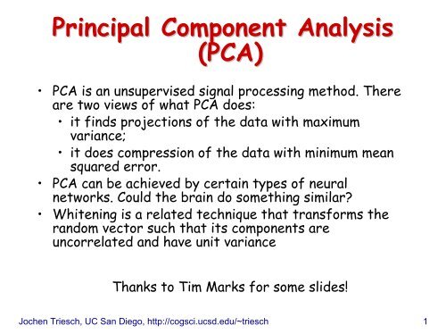
Principal Component Analysis (PCA)

Principal Component Analysis
(PCA)
• PCA is an unsupervised signal processing method. There
are two views of what PCA does:
• it finds projections of the data with maximum
variance;
• it does compression of the data with minimum mean
squared error.
• PCA can be achieved by certain types of neural
networks. Could the brain do something similar?
• Whitening is a related technique that transforms the
random vector such that its components are
uncorrelated and have unit variance
Thanks to Tim Marks for some slides!
Jochen Triesch, UC San Diego, http://cogsci.ucsd.edu/~triesch 1

Maximum Variance Projection
• Consider a random vector x with arbitrary joint pdf
• in PCA we assume that x has zero mean
• we can always achieve this by constructing x’=x-µ
• Scatter plot and projection y onto a “weight” vector w
w
y
n
T
= w x = ∑
i=
1
cos(
α )
• Motivating question: y is a scalar random variable that
depends on w; for which w is the variance of y maximal?
Jochen Triesch, UC San Diego, http://cogsci.ucsd.edu/~triesch 2
x
y
=
w
×
x
×
w
i
x
i

Example:
• consider projecting x onto the red w r and blue w b who
happen to lie along the coordinate axes in this case:
• clearly, the projection
onto w b has the higher
variance, but is there
a w for which it’s even
higher?
Jochen Triesch, UC San Diego, http://cogsci.ucsd.edu/~triesch 3
y
y
r
b
=
=
w
w
T
r
T
b
x
x
=
=
n
∑
i=
1
n
∑
i=
1
w
w
ri
bi
x
i
x
i

• First, what about the mean (expected value) of y?
y
=
w
T
x
=
• so we have:
n
∑
i=
1
n
i=
1
w
i
x
i
E(
y)
= E(
∑ w ) = ∑ ( ) = ∑
ixi
E wi
xi
wiE
( x
i=
1
since x has zero mean, meaning that E(x i ) = 0 for all i.
• This implies that the variance of y is just:
n
• Note that this gets arbitrarily big if w gets longer and
longer, so from now on we restrict w to have length 1,
i.e. (w T w) 1/2 =1
Jochen Triesch, UC San Diego, http://cogsci.ucsd.edu/~triesch 4
n
i=
1
( ( ) ) ) 2
2 ( 2
( ) ( w ) ) T
y − E y = E y E
var( y ) =
E
= x
i
)
=
0

• continuing with some linear algebra tricks:
var(
=
=
E
w
2 ( T 2
y)
= E(
y ) = E ( w x)
)
( T
w x)(
T
x w ) T
w ( T
= E xx )
T
C
x
w
where C x is the correlation matrix (or covariance
matrix) of x.
• We are looking for the vector w that maximizes this
expression
• Linear algebra tells us that the desired vector w is the
eigenvector of C x corresponding to the largest
eigenvalue
Jochen Triesch, UC San Diego, http://cogsci.ucsd.edu/~triesch 5
w

Reminder: Eigenvectors and Eigenvalues
• let A be an nxn (square) matrix. The n-component vector
v is an eigenvector of A with the eigenvalue λ if:
Av = λv
i.e. multiplying v by A only changes the length by a
factor λ but not the orientation.
Example:
• for the scaled identity matrix is every vector is an
eigenvector with identical eigenvalue s
⎛ s
⎜
⎜ M
⎜
⎝0
L
O
L
0⎞
⎟
M ⎟v
= sv
s ⎟
⎠
Jochen Triesch, UC San Diego, http://cogsci.ucsd.edu/~triesch 6

Notes:
• if v is an eigenvector of a matrix A then any scaled
version of v is an Eigenvector of A, too
• if A is a correlation (or covariance) matrix, then all the
eigenvalues are real and nonnegative; the eigenvectors
can be chosen to be mutually orthonormal:
v
T
i
v
k
= δ
ik
⎧1:
i = k
= ⎨
⎩0
: i ≠ k
(δ ik is the so-called Kronecker delta)
• also, if A is a correlation (or covariance) matrix, then A
is positive semidefinite:
T
v Av ≥ 0 ∀ v ≠
Jochen Triesch, UC San Diego, http://cogsci.ucsd.edu/~triesch 7
0

The PCA Solution
• The desired direction of maximum variance is the
direction of the unit-length eigenvector v1 of Cx with the
largest eigenvalue
• Next, we want to find the direction whose projection
has the maximum variance among all directions
perpendicular to the first eigenvector v1 . The solution to
this is the unit-length eigenvector v2 of Cx with the 2nd highest eigenvalue.
• In general, the k-th direction whose projection has the
maximum variance among all directions perpendicular to
the first k-1 directions is given by the k-th unit-length
eigenvector of Cx . The eigenvectors are ordered such
that:
λ ≥
1
≥ λ2
≥ Lλn−1
• We say the k-th principal component of x is given by:
y k =
Jochen Triesch, UC San Diego, http://cogsci.ucsd.edu/~triesch 8
v T
k
x
λ
n

What are the variances of the PCA projetions?
• From above we have:
( T 2 ) T
( x)
w C w
var( y ) = E =
w x
• Now utilize that w is the k-th eigenvector of C x :
var(
y)
=
=
v
v
T
k
T
k
C
x
v
k
=
( C v )
( ) T
λ k vk
= λk
vk
vk
= k
where in the last step we have exploited that v k has unit
length. Thus, in words, the variance of the k-th principal
component is simply the eigenvalue of the k-th
eigenvector of the correlation/covariance matrix.
Jochen Triesch, UC San Diego, http://cogsci.ucsd.edu/~triesch 9
v
T
k
x
k
λ

To summarize:
• The eigenvectors v 1 , v 2 , …, v n of the covariance matrix have
corresponding eigenvalues λ 1 ≥ λ 2 ≥ … ≥ λ n . They can be found
with standard algorithms.
• λ 1 is the variance of the projection in the v 1 direction, λ 2 is
the variance of the projection in the v 2 direction, and so on.
• The largest eigenvalue λ 1 corresponds to the principal
component with the greatest variance, the next largest
eigenvalue corresponds to the principal component with the
next greatest variance, etc.
• So, which eigenvector (green or red) corresponds to the
smaller eigenvalue in this example?
Jochen Triesch, UC San Diego, http://cogsci.ucsd.edu/~triesch 10

PCA for multinomial Gaussian
• We can think of the joint pdf of the multinomial
Gaussian in terms of the (hyper-) ellipsoidal (hyper-)
surfaces of constant values of the pdf.
• In this setting, principle component analysis (PCA) finds
the directions of the axes of the ellipsoid.
• There are two ways to think about what PCA does next:
• Projects every point perpendicularly onto the axes of
the ellipsoid.
• Rotates the ellipsoid so its axes are parallel to the
coordinate axes, and translates the ellipsoid so its
center is at the origin.
Jochen Triesch, UC San Diego, http://cogsci.ucsd.edu/~triesch 11

y
Two views of what PCA does
a) projects every point x onto the axes of
the ellipsoid to give projection c.
b) rotates space so that the ellipsoid lines up
with the coordinate axes, and translates
space so the ellipsoid’s center is at the
origin.
PC2
c 2
x
c 1
PC1
⎡x⎤
⎢ ⎥
⎣y⎦
Jochen Triesch, UC San Diego, http://cogsci.ucsd.edu/~triesch 12
x
→
c
⎡c
⎢
⎣c
1
2
⎤
⎥
⎦

Transformation matrix for PCA
• Let V be the matrix whose columns are the eigenvectors
of the covariance matrix, Σ.
• Since the eigenvectors v i are all normalized to have length
1 and are mutually orthogonal, the matrix V is orthonormal
(VV T = I), i.e. it is a rotation matrix
• the inverse rotation transformation is given by the
transpose V T of matrix V
⎡ ↑
⎢
⎢
⎢
⎣ ↓
v 1
↑
v
2
↓
V
L
↑
v
n
↓
⎤
⎥
⎥
⎥
⎦
⎡←
⎢
⎢
←
⎢
⎢
⎣←
→⎤
→
⎥
⎥
⎥
⎥
→⎦
Jochen Triesch, UC San Diego, http://cogsci.ucsd.edu/~triesch 13
V
v1 v
M
v
2
n
T

Transformation matrix for PCA
• PCA transforms the point x (original coordinates) into the
point c (new coordinates) by subtracting the mean from x
(z = x – m) and multiplying the result by V T
⎡←
⎢
⎢
←
⎢
⎢
⎣←
V
v1
v2
M
v
n
T
→⎤
→
⎥
⎥
⎥
⎥
→⎦
⎡↑⎤
⎢ ⎥
⎢z
⎥
⎢ ⎥
⎣↓⎦
• this is a rotation because V T is an orthonormal matrix
• this is a projection of z onto PC axes, because v 1 • z is
projection of z onto PC1 axis, v 2 • z is projection onto PC2
axis, etc.
z
Jochen Triesch, UC San Diego, http://cogsci.ucsd.edu/~triesch 14
=
⎡v
⎢
⎢
v
⎢
⎢
⎣v
1
2
n
c
M
⋅
⋅
⋅
z⎤
z
⎥
⎥
⎥
⎥
z⎦

• PCA expresses the mean-subtracted point, z = x – m, as a
weighted sum of the eigenvectors vi . To see this, start
with:
T
⎡←
⎢
⎢
←
⎢
⎢
⎣←
V
v
v
1
2
M
v
D
→⎤
→
⎥
⎥
⎥
⎥
→⎦
• multiply both sides of the equation from the left by V:
VV T z = Vc | exploit that V is orthonormal
z = Vc | i.e. we can easily reconstruct z from c
z
⎡↑⎤
⎢ ⎥
⎢z
⎥
⎢ ⎥
⎣↓⎦
=
=
⎡ ↑
⎢
⎢v
⎢
⎣ ↓
1
↑
v
2
↓
V
c
⎡c1
⎤
↑ ⎤ ⎢ ⎥
⎥ ⎢
c2
v ⎥
n ⎥ ⎢ M ⎥
↓ ⎥
⎦ ⎢ ⎥
⎣cn
⎦
Jochen Triesch, UC San Diego, http://cogsci.ucsd.edu/~triesch 15
z
⎡↑⎤
⎢ ⎥
⎢z
⎥
⎢ ⎥
⎣↓⎦
=
c
=
⎡ ↑ ⎤
⎢ ⎥
⎢v1
⎥
⎢ ⎥
⎣ ↓ ⎦
c
⎡ c
⎢
⎢
c
⎢ M
⎢
⎣c
+
1
2
D
⎤
⎥
⎥
⎥
⎥
⎦
c
⎡ ↑
⎢
⎢v
⎢
⎣ ↓
L 1
2 2
⎤
⎥
⎥
⎥
⎦
+
L
+
c
n
⎡ ↑
⎢
⎢v
⎢
⎣ ↓
n
⎤
⎥
⎥
⎥
⎦

PCA for data compression
What if you wanted to transmit someone’s height and weight,
but you could only give a single number?
• Could give only height, x
— = (uncertainty when height is known)
• Could give only weight, y
— = (uncertainty when weight is known)
• Could give only c 1 ,
the value of first PC
— = (uncertainty when first PC is known)
• Giving the first PC minimizes
the squared error of the result.
weight
Jochen Triesch, UC San Diego, http://cogsci.ucsd.edu/~triesch 16
y
PC2
To compress n-dimensional data into k dimensions, order the
principal components in order of largest-to-smallest
eigenvalue, and only save the first k components.
c 2
x
c 1
PC1
height

• Equivalent view: To compress n-dimensional data into k

PCA vs. Discrimination
• variance maximization or compression are different from
discrimination!
• consider this data coming stemming from two classes?
• which direction has max. variance, which discriminates
between the two clusters?
Jochen Triesch, UC San Diego, http://cogsci.ucsd.edu/~triesch 18

Application: PCA on face images
• 120 × 100 pixel grayscale 2D images of faces. Each
image is considered to be a single point in face space (a
single sample from a random vector):
⎡↑⎤
⎢ ⎥
⎢x⎥
⎢ ⎥
⎣↓⎦
• How many dimensions is the vector x ?
n = 120 • 100 = 12000
• Each dimension (each pixel) can take values between 0
and 255 (8 bit grey scale images).
• You can easily visualize points in this 12000 dimensional
space!
Jochen Triesch, UC San Diego, http://cogsci.ucsd.edu/~triesch 19

The original images (12 out of 97)
Jochen Triesch, UC San Diego, http://cogsci.ucsd.edu/~triesch 20

The mean face
Jochen Triesch, UC San Diego, http://cogsci.ucsd.edu/~triesch 21

• Let x 1 , x 2 , …, x p be the p sample images (n-dimensional).
• Find the mean image, m, and subtract it from each
image: z i = x i – m
• Let A be the matrix whose columns are the
mean-subtracted sample images.
⎡ ↑ ↑ ↑ ⎤
⎢
⎥
A = ⎢z1
z 2 L z p ⎥ n ×
⎢
⎥
⎣ ↓ ↓ ↓ ⎦
• Estimate the covariance matrix:
Σ
=
1
Cov( A)
= A A
p −1
What are the dimensions of Σ ?
matrix
Jochen Triesch, UC San Diego, http://cogsci.ucsd.edu/~triesch 22
T
p

The transpose trick
The eigenvectors of Σ are the principal component directions.
Problem:
• Σ is a nxn (12000×12000) matrix. It’s too big for us to
find its eigenvectors numerically. In addition, only the
first p eigenvalues are useful; the rest will all be zero,
because we only have p samples.
Solution: Use the following trick.
• Eigenvectors of Σ are eigenvectors of AA T ; but instead
of eigenvectors of AA T , the eigenvectors of A T A are easy
to find
What are the dimensions of A T A ? It’s a p×p matrix: it’s easy
to find eigenvectors since p is relatively small.
Jochen Triesch, UC San Diego, http://cogsci.ucsd.edu/~triesch 23

• We want the eigenvectors of AA T , but instead we calculated
the eigenvectors of A T A. Now what?
• Let v i be an eigenvector of A T A, whose eigenvalue is λ i
(ATA)vi = ? λivi A (ATAv ) i = A(λivi) AAT (Av ) i = λi (Avi) • Thus if v i is an eigenvector of A T A ,
Av i is an eigenvector of AA T , with the same eigenvalue.
Av 1 , Av 2 , … , Av n are the eigenvectors of Σ.
u 1 = Av 1 , u 2 = Av 2 , …, u n = Av n are called eigenfaces.
Jochen Triesch, UC San Diego, http://cogsci.ucsd.edu/~triesch 24

Eigenfaces
• Eigenfaces (the principal component directions of face
space) provide a low-dimensional representation of any
face, which can be used for:
• Face image compression and reconstruction
• Face recognition
• Facial expression recognition
Jochen Triesch, UC San Diego, http://cogsci.ucsd.edu/~triesch 25

The first 8 eigenfaces
Jochen Triesch, UC San Diego, http://cogsci.ucsd.edu/~triesch 26

PCA for low-dimensional low dimensional face
representation
• To approximate a face using only k dimensions, order the
eigenfaces in order of largest-to-smallest eigenvalue,
and only use the first k eigenfaces.
z
⎡↑⎤
⎢ ⎥
⎢z
⎥
⎢ ⎥
⎣↓⎦
=
=
⎡ ↑
⎢
⎢u1
⎢
⎣ ↓
⎡←
⎢
⎢←
⎢
⎣←
U
u
u
u
1
2
M
k
T
→⎤
⎥
→⎥
⎥
→⎦
U c
↑
u2
↓
L
⎡c1
⎤
↑ ⎤ ⎢ ⎥
⎥ ⎢
c2
u ⎥
k ⎥ ⎢ M ⎥
↓ ⎥
⎦ ⎢ ⎥
⎣ck
⎦
⎡ ↑ ⎤ ⎡ ↑ ⎤
⎢ ⎥ ⎢ ⎥
= c1
⎢u1
⎥ + c2
⎢u2
⎥ + L
⎢ ⎥ ⎢ ⎥
⎣ ↓ ⎦ ⎣ ↓ ⎦
⎡ ↑ ⎤
⎢ ⎥
⎢uk
⎥
⎢ ⎥
⎣ ↓ ⎦
Jochen Triesch, UC San Diego, http://cogsci.ucsd.edu/~triesch 27
⎡↑⎤
⎢ ⎥
⎢z
⎥
⎢ ⎥
⎣↓⎦
• PCA approximates a mean-subtracted face, z = x – m, as
a weighted sum of the first k eigenfaces:
z
=
c
⎡c
⎢
⎢c
M ⎢
⎣c
1
2
k
⎤
⎥
⎥
⎥
⎦
+
c
k

• To approximate the actual face we have to add the mean
face m to the reconstruction of z:
x
=
= U c + m
=
=
z + m
⎡ ↑
⎢
⎢u1
⎢
⎣ ↓
c
1
↑
u
2
↓
⎡ ↑ ⎤
⎢ ⎥
⎢u1
⎥ +
⎢ ⎥
⎣ ↓ ⎦
⎡c1
⎤
↑ ⎤ ⎢ ⎥ ⎡↑
⎤
⎥ ⎢
c2
⎢ ⎥
L u ⎥
k ⎥ + ⎢m
⎢ M ⎥ ⎥
↓ ⎥ ⎢ ⎥
⎦ ⎢ ⎥ ⎣↓
⎦
⎣ck
⎦
⎡ ↑ ⎤ ⎡ ↑ ⎤ ⎡↑
⎤
⎢ ⎥ ⎢ ⎥ ⎢ ⎥
c2
⎢u
2 ⎥ + L + ck
⎢u
k ⎥ + ⎢m⎥
⎢ ⎥ ⎢ ⎥ ⎢ ⎥
⎣ ↓ ⎦ ⎣ ↓ ⎦ ⎣↓
⎦
• The reconstructed face is simply the mean face with
some fraction of each eigenface added to it
Jochen Triesch, UC San Diego, http://cogsci.ucsd.edu/~triesch 28

The mean face
Jochen Triesch, UC San Diego, http://cogsci.ucsd.edu/~triesch 29

Approximating a face using the
first 10 eigenfaces
Jochen Triesch, UC San Diego, http://cogsci.ucsd.edu/~triesch 30

Approximating a face using the
first 20 eigenfaces
Jochen Triesch, UC San Diego, http://cogsci.ucsd.edu/~triesch 31

Approximating a face using the
first 40 eigenfaces
Jochen Triesch, UC San Diego, http://cogsci.ucsd.edu/~triesch 32

Approximating a face using all
97 eigenfaces
Jochen Triesch, UC San Diego, http://cogsci.ucsd.edu/~triesch 33

Notes:
• not surprisingly, the approximation of the reconstructed
faces get better when more eigenfaces are used
• In the extreme case of using no eigenface at all, the
reconstruction of any face image is just the average
face
• In the other extreme of using all 97 eigenfaces, the
reconstruction is exact, since the image was in the
original training set of 97 images. For a new face image,
however, its reconstruction based on the 97 eigenfaces
will only approximately match the original.
• What regularities does each eigenface capture? See
movie.
Jochen Triesch, UC San Diego, http://cogsci.ucsd.edu/~triesch 34

Eigenfaces in 3D
• Blanz and Vetter (SIGGRAPH ’99). The video can be
found at:
http://graphics.informatik.uni-freiburg.de/Sigg99.html
Jochen Triesch, UC San Diego, http://cogsci.ucsd.edu/~triesch 35