TARIFF AGREEMENTS AND NON-RENEWABLE RESOURCE ... - Ivie
Create successful ePaper yourself
Turn your PDF publications into a flip-book with our unique Google optimized e-Paper software.
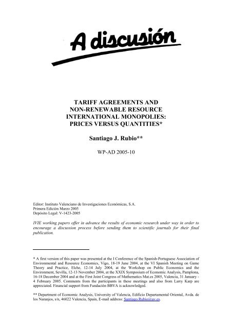
<strong>TARIFF</strong> <strong>AGREEMENTS</strong> <strong>AND</strong><br />
<strong>NON</strong>-<strong>RENEWABLE</strong> <strong>RESOURCE</strong><br />
INTERNATIONAL MONOPOLIES:<br />
PRICES VERSUS QUANTITIES*<br />
Santiago J. Rubio**<br />
WP-AD 2005-10<br />
Editor: Instituto Valenciano de Investigaciones Económicas, S.A.<br />
Primera Edición Marzo 2005<br />
Depósito Legal: V-1423-2005<br />
IVIE working papers offer in advance the results of economic research under way in order to<br />
encourage a discussion process before sending them to scientific journals for their final<br />
publication.<br />
* A first version of this paper was presented at the I Conference of the Spanish-Portuguese Association of<br />
Environmental and Resource Economics, Vigo, 18-19 June 2004, at the VI Spanish Meeting on Game<br />
Theory and Practice, Elche, 12-14 July 2004, at the Workshop on Public Economics and the<br />
Environment, Sevilla, 12-13 November 2004, at the XXIX Symposium of Economic Analysis, Pamplona,<br />
16-18 December 2004 and at the First Joint Congress of Mathematics Mat.es 2005, Valencia, 31 January -<br />
4 February 2005. Comments from the participants in these meetings and also from Larry Karp are<br />
appreciated. Financial support from Fundación BBVA is acknowledged.<br />
** Department of Economic Analysis, University of Valencia, Edificio Departamental Oriental, Avda. de<br />
los Naranjos, s/n, 46022 Valencia, Spain, E-mail address: Santiago.Rubio@uv.es.
<strong>TARIFF</strong> <strong>AGREEMENTS</strong> <strong>AND</strong><br />
<strong>NON</strong>-<strong>RENEWABLE</strong> <strong>RESOURCE</strong> INTERNATIONAL MONOPOLIES:<br />
PRICES VERSUS QUANTITIES<br />
Santiago J. Rubio<br />
ABSTRACT<br />
In this paper we model the case of an international non-renewable resource<br />
monopolist as a differential game between the monopolist and the governments of<br />
the importing countries, and we investigate whether a tariff on the resource<br />
importations can be advantageous for the importing countries. We find that the<br />
results depend crucially on the kind of strategies the importing country governments<br />
can play and on whether the monopolist chooses the price or the extraction rate. For<br />
a price-setting monopolist it is shown that the importing countries cannot use a tariff<br />
to capture monopoly rents if they are constrained to use open-loop strategies, even if<br />
the governments sign a tariff agreement. This result is drastically modified if the<br />
importing countries in the tariff agreement use Markov (feedback) strategies. For a<br />
quantity-setting monopolist the nature of the game changes and an open-loop tariff<br />
is advantageous for the importing countries. Moreover, in this case the importing<br />
countries in a tariff agreement enjoy a strategic advantage which allows them to<br />
behave as a leader.<br />
Keywords: tariffs, tariff agreements, non-renewable resources, depletion effects,<br />
price-setting monopolist, quantity-setting monopolist, differential games, open-loop<br />
strategies, linear strategies, Markov-perfect Nash equilibrium, Markov-perfect<br />
Stackelberg equilibrium.<br />
JEL Classification Numbers: C73, D41, D42, F02, H20, Q38.<br />
2
1 Introduction<br />
The issue of using an import tariff to capture non-renewable resource rents<br />
was addressed sometime ago in a nice piece of work by Bergstrom (1982).<br />
In his paper, he shows that if all importing countries of a competitively<br />
supplied non-renewable resource select the same ad valorem tariff on the resource<br />
consumed at any time, the tariff is advantageous for the importing<br />
countries in the sense that they capture resource rents from the exporting<br />
countries. He characterizes the Nash equilibrium of the game among the<br />
importing countries by a simple rule relating the equilibrium ad valorem<br />
tariff to demand elasticities and market shares. In the second part of the<br />
paper, he argues that almost all the profits of a monopolist can be taxed<br />
away by the importing countries if they choose a sufficiently high tariff as<br />
long as the profit-maximizing level of the monopolist’s price is independent<br />
of the tariff. These results are obtained for a Hotelling-type model with a<br />
costlessly extracted non-renewable resource. Later, several papers addressed<br />
this issue, see Brander and Djajic (1983), Karp (1984), Maskin and Newbery<br />
(1990), Karp and Newbery (1991, 1992). 1 Among them only Brander and<br />
Djajic (1983) and Karp (1984) have addressed this issue for the case of a<br />
non-renewable resource monopoly. Brander and Djajic develop their analysis<br />
in the context of a simple two-country general equilibrium model of trade<br />
in exhaustible resources where it is assumed that the resource is extracted<br />
costlessly and used as an essential input in the production of a homogeneous<br />
consumption good. They find that the country without resource has an incentivetoimposeatariff<br />
so as to extract at least some of the available rent.<br />
Themagnitudeoftheoptimaltariff isfoundtobeanincreasingfunction<br />
of the relative size of the importing country and approaches the confiscatory<br />
level as the resource importing country becomes very large. In Karp the interaction<br />
between a monopolist and a single buyer is modeled as a Stackelberg<br />
game where the extraction cost is inversely related to the stock (depletion effects)<br />
and the buyer is the leader of the game. The buyer chooses a tariff and<br />
the monopolist the rate of extraction. He shows that the open-loop tariff is<br />
temporally inconsistent because of the stock-dependence of extraction costs.<br />
Besides, he proposes a method of obtaining temporally consistent strategies<br />
and concludes that the consistent tariff against the monopolist is in general<br />
1 A recent contribution by Hörner and Kamien (2004) shows that the intertemporal<br />
no-arbitrage condition that arises if the durable good monopolist seller can commit to a<br />
price path mirrors the intertemporal no-arbitrage condition if the monopsonist buyer of<br />
an exhaustible resource supplied by competitive sellers can commit to a profile of import<br />
tariffs. The time-consistency of the tariff in this case has been studied by Kemp and Long<br />
(1980) and Karp (1984, 1991).<br />
3
not identically zero which implies that the consistent tariff allows the buyer<br />
to improve his position. 2<br />
In the firstpartofthepaperwemodelthecaseofaprice-settingmonopolist<br />
selling to noncooperative consuming nations, first studied by Bergstrom<br />
(1982), as a differential game. In the second part, we analyze the case of<br />
a quantity-setting monopolist. Moreover, we also extend his analysis by assuming<br />
that extraction cost is directly related to accumulated extractions<br />
(depletion effects).<br />
Contrary to the results obtained by Bergstrom (1982), we find that the<br />
profit-maximizing level of the monopolist’s price is not independent of the<br />
tariff andthattheopen-loopNashequilibriumtariff is zero. This result<br />
appears because the user cost for the importing countries is equal to the tariff<br />
times the monopoly price and because the extraction cost is supported by the<br />
monopolist. In this case the user cost for importing countries must increase<br />
at a rate equal to the interest rate but this is incompatible with the fact<br />
that ultimately the rent must be zero because of the economic exhaustion<br />
of the resource. We also find that this result applies for a per unit tariff<br />
and when the importing countries cooperate imposing the same tariff rate<br />
on the resource importations, i.e., when the importing country governments<br />
sign a tariff agreement, and independently of whether it is assumed that the<br />
countries are symmetric or not.<br />
In order to clarify whether this result is a consequence of the equilibrium<br />
concept used to solve the game, we propose a differential game between a<br />
monopolist and a coalition of importing country governments for which it is<br />
possible to calculate the stationary linear Markov strategies. The solution<br />
to this game establishes that the importing countries can capture part of the<br />
monopoly’s rents for their consumer using a tariff on the resource importations.<br />
Thus, we find that when the monopolist chooses a pricing policy the<br />
tariff is advantageous for the importing countries if the importing countries<br />
co-operate through a tariff agreement and the optimal policy is defined using<br />
a feedback strategy.<br />
For the case of a quantity-setting monopolist, as the importing countries<br />
have no influence on the dynamics of the stock, the game among the importing<br />
countries becomes, in fact, a static game and given the influence of<br />
the tariff rate on the monopoly price the importing countries find it advan-<br />
2 He proposes an alternative method to the one developed by Simaan and Cruz (1973),<br />
see Prop.2 in Karp’s paper. Simaan and Cruz’s method is for the leader to treat the<br />
follower’s dynamic programming equation as a constraint, and to solve his own problem<br />
using dynamic programing methods. This “backward” method of solution eliminates at<br />
each point all control rules that are not optimal given the state at the time, and results<br />
in consistent control rules.<br />
4
tageous to set a tariff on the resource importations. 3 On the other hand,<br />
if the governments of the importing countries sign a tariff agreement it is<br />
pretty obvious that the open-loop Nash equilibrium policy is to choose, for<br />
a given extraction rate, a tariff such that the monopolist’s price be zero, but<br />
then the monopoly is not interested in exploiting the resource so that finally<br />
the consumers of the importing countries are not going to enjoy any surplus.<br />
However, the coalition has another alternative since the importing country<br />
governments, in fact, enjoy a strategic advantage given that they can influence<br />
the monopoly price through the tariff. In other words, the importing<br />
country governments have another alternative because the coalition can behave<br />
as a leader. 4 To conclude the analysis we calculate, following the Simaan<br />
and Cruz’s (1973) method, the stationary Markov-perfect Stackelberg equilibrium<br />
in linear strategies which guarantees the strong time consistency of<br />
the tariff, and we obtain that the importing countries are interested in setting<br />
a tariff that provides the monopoly with the possibility of obtaining a<br />
positive price with the aim of getting a positive surplus for their consumers.<br />
A policy that clearly is superior to the one derived from the open-loop Nash<br />
equilibrium.<br />
The paper is organized as follows. In Section 2 the case of a price-setting<br />
monopolist is studied and the case of a quantity-setting monopolist is dealt<br />
with in Section 3. The comparison between the Markov-perfect Nash equilibrium<br />
of the differential game where the monopolist sets up the price and<br />
the Markov-perfect Stackelberg equilibrium where the monopolist sets up<br />
the extraction rate appears in Section 4. Conclusions and subjects for future<br />
research are presented in Section 5.<br />
2 The Case of a Price-setting Monopolist<br />
As in Bergstrom’s (1982) analysis, we shall confine ourselves to a partial equilibrium<br />
model. Assuming that the representative consumer of the importing<br />
country acts as a price-taker agent, we can write the consumer’s welfare function<br />
as U i (q i ) − p(1 + θ i )q i + R i , where U i (q i ) is the consumer’s gross surplus,<br />
q i the amount of the resource bought by the representative consumer of the<br />
importing country i, p the international price of the resource, θ i the “ad<br />
valorem” tariff rate on the resource imports fixed by the government of the<br />
importing country i, andR i a lump-sum transfer that the consumer receives<br />
3 This is the same result as the one obtained by Karp and Newbery (1991) when competitive<br />
suppliers move first in the game. However, we get it here as a consequence of the<br />
fact that the monopolist uses the extraction rate as a control variable.<br />
4 This is the hypothesis explored by Karp (1984).<br />
5
from the government. Thus, the resource demand depends only on the consumer<br />
price: Ui(q i )=p(1 + θ i ) and the demand function can be written as<br />
q i = D i (p(1 + θ i )) with Di < 0 if the marginal utility is decreasing. 5 Thus<br />
the aggregate demand is Q = n<br />
i=1 D i(p(1 + θ i )).<br />
The governments set the tariff with the aim of maximizing the discounted<br />
present value of the representative consumer’s welfare. They reimburse tariff<br />
revenues as lump-sum transfers, sothatfinally the consumer’s welfare does<br />
not depend on tariff revenues. The optimal time path for the tariff is thus<br />
given by the solution of the following optimal control problem<br />
max<br />
{θ i }<br />
∞<br />
0<br />
e −rt (U i (D i (p(1 + θ i ))) − pD i (p(1 + θ i ))) dt, i =1, ..., n. (1)<br />
where r is the discount rate.<br />
On the other side of the market we have a monopoly extracting the resource<br />
at an aggregate cost equal to c(x)Q, where c(x) is the marginal extraction<br />
cost, with c > 0 and c ≥ 0, xstands for the accumulated extractions<br />
and Q for the current extraction rate of the resource. The objective of the<br />
monopoly is to define a price strategy that maximizes the present value of<br />
profits<br />
max<br />
{p}<br />
∞<br />
0<br />
e −rt (p − c(x))<br />
<br />
n<br />
D i (p(1 + θ i )) dt. (2)<br />
Given the price the extraction rate is determined by the demand function so<br />
that the dynamics of the accumulated extractions is<br />
n<br />
ẋ = Q = D i (p(1 + θ i )), x(0) = x 0 ≥ 0. (3)<br />
i=1<br />
Both types of players face the same dynamic constraint and the optimal<br />
time paths for the tariff and the price are given by the solution of the differential<br />
game between the monopolist and the n importing countries defined<br />
by (1) − (2) − (3).<br />
i=1<br />
2.1 TheOpen-loopNashEquilibrium<br />
First, we write the Hamiltonian associated to the optimal control problems<br />
of the importing countries.<br />
5 Di stands for the derivative of the demanded quantity with respect to the consumer<br />
price: p(1 + θ i ).<br />
6
H i = U i (D i (p(1 + θ i ))) − pD i (p(1 + θ i )) + λ i<br />
which yields the following necessary conditions<br />
n<br />
D j (p(1 + θ j )),<br />
j=1<br />
pθ i = −λ i , ˙λi = rλ i , (4)<br />
which establish that for a given value of the co-state variable the price is a<br />
strategic substitute of the tariff rate. Notice that now, as the extraction costs<br />
are supported directly by the monopolist, the tariff, pθ i , must increase at the<br />
interest rate.<br />
For the monopolist the Hamiltonian is<br />
H M =(p − c(x)+λ M )<br />
and the necessary conditions are<br />
n<br />
D i (p(1 + θ i )),<br />
i=1<br />
n<br />
n<br />
D i +(p − c + λ M ) (1 + θ i )Di =0, (5)<br />
i=1<br />
i=1<br />
˙λ M = rλ M + c <br />
n<br />
D i , (6)<br />
i=1<br />
where (5) is the instantaneous reaction function of the monopoly. By differentiation<br />
we can obtain that<br />
∂p pDi +(p − c + λ M )(Di + p(1 + θ i ) Di )<br />
= −<br />
∂θ i 2 n<br />
i=1 (1 + θ i)Di +(p − c + λ M) n<br />
i=1 (1 + θ i) 2 Di<br />
<br />
< 0, (7)<br />
and so we can establish that if the demand functions are concave, the tariff<br />
rate of one importing country is also a strategic substitute of the monopoly<br />
price for given values of the state and co-state variables.<br />
With D <br />
i<br />
≤ 0, the numerator and the denominator of (7) are negative<br />
since by (5) (p − c + λ M ) must be positive. Moreover, it is easy to check that<br />
(5) is the standard condition that characterizes the monopoly equilibrium:<br />
7
marginal revenue equal to marginal cost, now including the user cost of the<br />
resource. (5) can be written as<br />
n<br />
i=1 D i<br />
n<br />
i=1 (1 + θ i)D i<br />
+ p = c − λ M ,<br />
and taking common factor p as<br />
1<br />
MR = p +1 = c − λ M = MC,<br />
ε Q,p<br />
where ε Q,p is the elasticity of the aggregate demand function.<br />
The open-loop Nash equilibrium is given by the solution to the following<br />
system of 2n +3equations.<br />
pθ i = −λ i , i =1, ..., n, (8)<br />
˙λ i = rλ i ,i=1, .., n, (9)<br />
0 =<br />
n<br />
n<br />
D i +(p − c + λ M ) (1 + θ i )Di, (10)<br />
i=1<br />
n<br />
˙λ M = rλ M + c D i , (11)<br />
ẋ =<br />
i=1<br />
i=1<br />
n<br />
D i . (12)<br />
i=1<br />
In order to calculate the steady state we have to take into account that<br />
the different countries can have different backstop prices. In this case, what is<br />
going to occur is that the countries are going to leave the market sequentially<br />
as the monopoly price reaches its backstop price so that the steady state<br />
will be defined by θ ∞ i = λ ∞ i = λ ∞ M =0, i =1,...,n, p ∞ = c(x ∞ ) and<br />
D j (p ∞ )=0where j is the country with the highest backstop price. Then it<br />
is straightforward that<br />
Proposition 1 The governments of the importing countries cannot capture<br />
theresourcerentusingatariff, in other words, the open-loop Nash equilibrium<br />
tariff rate with depletion effects is zero.<br />
This is an immediate consequence of the fact that the tariff, pθ i , must<br />
increase at a constant rate which is incompatible with the fact that ultimately<br />
the tariff rate must be zero because of the economic exhaustion of<br />
the resource. Notice that the price cannot be zero since at the steady state<br />
it is equal to the marginal extraction cost. Thus the unique path that can<br />
8
converge to the steady state requires that θ i = λ i =0throughout the exploitation<br />
period of the resource and then the system (8)-(9)-(10)-(11)-(12)<br />
yields the standard solution for the monopolistic extraction with depletion<br />
effects. As long as this argument does not depend on the cost structure, the<br />
result will also be valid when there are no depletion effects. It will be valid as<br />
well even if the importing countries cooperate imposing the same tariff rate<br />
on the resource importations, i.e., even if the importing country governments<br />
sign a tariff agreement and independently of whether we assume that they<br />
are symmetric or not. It is easy to show that the previous result also applies<br />
to the case of a per unit tariff sincealltheanalysisfortheperunittariff is<br />
identical to the one developed in this section simply substituting pθ i by the<br />
per unit tariff.<br />
2.2 A Tariff Agreement: The Markov-perfect Nash<br />
Equilibrium<br />
Next, we want to investigate whether this last result is a consequence of the<br />
equilibrium concept used to solve the game. To do so we propose in this<br />
section a game for which it is possible to calculate the stationary Markovian<br />
(feedback) strategies. Now we assume that the governments of the importing<br />
countries sign an agreement to impose the same per unit tariff on the resource<br />
importations with the aim of maximizing the discounted present value of the<br />
sum of the aggregate consumer’s welfare. 6 In order to obtain an analytical<br />
solution for the game we also assume that the consumer’s gross surplus is<br />
given by U i (q i )=aq i − (1/2)qi 2 and that the extraction cost is linear, c(x) =<br />
cx. With these changes we have a differential game between a monopolist<br />
and a coalition of the importing country governments that can be written as<br />
follows for the monopolist,<br />
max<br />
{p}<br />
∞<br />
0<br />
e −rt ((p − cx)n(a − p − θ)) dt, (13)<br />
and as follows for the coalition of the governments of the importing countries<br />
max<br />
{θ}<br />
∞<br />
0<br />
e −rt n<br />
(a − p)(a − p − θ) − 1 <br />
2 (a − p − θ)2 dt, (14)<br />
6 As we have obtained the same qualitative results both for an ad valorem tariff and<br />
foraperunittariff, the change in the specification of the tariff does not suppose a strong<br />
discontinuity in the analysis developed in this paper. Besides, a per unit tariff allows us<br />
to compute the Markov-perfect Nash equilibrium in linear strategies.<br />
9
the dynamic constraint being<br />
s.t. ẋ = Q = n(a − p − θ), x(0) = x 0 ≥ 0. (15)<br />
Markov strategies must satisfy the following system of Hamilton-Jacobi-<br />
Bellman equations:<br />
<br />
rW A = max n<br />
(a − p)(a − p − θ) − 1 <br />
{θ}<br />
2 (a − p − θ)2<br />
+W An(a − p − θ)} , (16)<br />
rW M = max<br />
{p} {(p − cx)n(a − p − θ)+W Mn(a − p − θ)} , (17)<br />
where W M (x) stands for the optimal current value functions associated with<br />
the dynamic optimization problem for the monopoly (13) and W A (x) for the<br />
optimal current value functions associated with the dynamic optimization<br />
problem for the agreement (14); i.e., they denote the maxima of the objectives<br />
(13) and (14) subject to (15) for the current value of the state variable.<br />
From the first-order conditions for the maximization of the right-hand<br />
sides of the HJB equations, we get the instantaneous reaction functions of<br />
the governments and the monopolist:<br />
θ = −W A, (18)<br />
p = 1 2 (a + cx − W M − θ) . (19)<br />
These expressions establish that the optimal tariff is independent of the<br />
monopoly price and equal, as before, to the user cost of the resource for the<br />
importing countries, and that the price and the tariff are strategic substitutes<br />
for the monopolist.<br />
By substitution of (18) and (19), we get the solution of the price as a function<br />
of the first derivatives of the value functions: p = 1 2 (a + cx − W M + W A ) .<br />
Next, by incorporating the optimal strategies into the HJB Eqs. (16) and<br />
(17), we eliminate the maximization and obtain, after some calculations, a<br />
pair of nonlinear differential equations:<br />
rW A = n 8 (a − cx + W M + W A) 2 , (20)<br />
rW M = n 4 (a − cx + W M + W A) 2 . (21)<br />
In order to derive the solution to this system of differential equations, we<br />
guess quadratic representations for the value functions W A and W M ,<br />
10
W A (x) = 1 2 α Ax 2 + β A x + µ A ,W M (x) = 1 2 α Mx 2 + β M x + µ M , (22)<br />
and we apply the same procedure as the one used by Wirl and Dockner (1995)<br />
to calculate the coefficients, see Appendix A. Substituting these coefficients in<br />
(18) and (19), we obtain the linear Markov-perfect Nash equilibrium strategies<br />
for the tariff and the price:<br />
where<br />
θ =<br />
p =<br />
anδ<br />
4r +3nδ − nδ2 x,<br />
4r<br />
(23)<br />
2a(r + nδ)<br />
4r +3nδ + 2c + δ x,<br />
6<br />
(24)<br />
δ = 2 3cnr + r<br />
2 0.5 − r<br />
> 0.<br />
3n<br />
By visual inspection it can be seen that the tariff is inversely related to<br />
the accumulated extractions whereas the price increases with the exploitation<br />
of the resource. Now using the equilibrium strategies, differential equation<br />
(15) can be solved, yielding<br />
x =(x 0 − a <br />
c )exp − nδ <br />
2 t + a c , (25)<br />
and by substitution in the equilibrium strategies the tariff and price dynamics<br />
are obtained. 7<br />
<br />
θ = anδ2<br />
4rc exp − nδ <br />
2 t ,p= a 1 − 2c + δ <br />
exp − nδ <br />
6c 2 t . (26)<br />
Finally, the consumer price can be simply calculated by the addition of<br />
the monopoly price and tariff.<br />
π = θ + p = a<br />
1 − δ <br />
2c exp − nδ <br />
2 t (27)<br />
so we can summarize these results as<br />
7 In order to simplify the presentation we assume that x 0 =0. This does not change<br />
the sign of the dynamics of these two variables.<br />
11
Remark 1 The Markov-perfect Nash equilibrium tariff rate decreases throughout<br />
the exploitation period of the resource and converges to zero in the long<br />
run. Moreover, the monopoly and consumer prices are increasing and convergetothebackstopprice.<br />
Clearly, these results establish that the commitment that the open-loop<br />
Nash equilibrium requires for the importing countries, a commitment for the<br />
entire exploitation period of the resource, drastically reduces the possibilities<br />
of using a tariff to capture part of the monopoly’s rents. In other words,<br />
the importing country governments have to play feedback strategies, i.e., to<br />
define the optimal policy as a function of the accumulated extractions, in<br />
order to be able to impose an advantageous tariff for the consumers.<br />
Finally, we obtain the following value functions for the agreement and the<br />
monopoly<br />
W A (x) = nδ2<br />
8r x2 −<br />
anδ<br />
4r +3nδ x +<br />
2a2 nr<br />
(4r +3nδ) 2 ,W M(x) =2W A (x). (28)<br />
3 The Case of a Quantity-setting Monopolist<br />
Until now we have assumed that the monopoly chooses the price and the<br />
market establishes the resource extraction rate. In this section we analyze<br />
the other possibility the monopoly has: to choose the quantity and leave the<br />
market to set up the price. In this case by substitution of the inverse demand<br />
function in the instantaneous consumer’s welfare the following expression is<br />
obtained<br />
W i = U i<br />
<br />
Di<br />
<br />
p(Q, ¯θ (1 + θi )) − p(Q, ¯θ)D i<br />
<br />
p(Q, ¯θ)(1 + θi ) , (29)<br />
where ¯θ is the vector of the tariff rates.<br />
Astheextractionrateisdeterminedbythemonopolist,thegovernments<br />
of the importing countries have no influence on the dynamics of the stock.<br />
For this reason, in this case the tariff rate is given by the Nash equilibrium<br />
ofthestaticgamedefined by (29). In other words, at each point in time the<br />
importingcountrieschooseatariff rate to maximize the instantaneous flow<br />
of the consumer’s welfare given the extraction rate and the rival’s tariff rates.<br />
The first order conditions yield<br />
(U i − p)D i<br />
<br />
∂p<br />
(1 + θ i )+p<br />
∂θ i<br />
= ∂p<br />
∂θ i<br />
D i , i =1, ..., n,<br />
12
and as Ui = p(1 + θ i ) the following expression is obtained<br />
<br />
∂p<br />
pθ i Di<br />
(1 + θ i )+p = ∂p D i .<br />
∂θ i ∂θ i<br />
By differentiation of the demand function we get<br />
∂p<br />
D<br />
= − ip<br />
<br />
∂θ n<br />
i j=1 D j (1 + θ j)<br />
that by substitution into the above expression yields<br />
D i<br />
pθ i = −j=i D j (1 + θ , i =1, ..., n. (30)<br />
j)<br />
This is the version for an “ad valorem” tariff of the one obtained by Karp<br />
and Newbery (1991, p. 288) for a per unit tariff.<br />
Assuming that the system (30) has a unique solution, the dynamic of the<br />
extraction rate and hence the dynamics of the tariff rate can be calculated as<br />
the solution of a standard optimal control problem. 8 This result shows that<br />
the nature of the game changes when the monopoly sets the quantity instead<br />
of the price. Now at each moment, given the extraction rate, the importing<br />
countries can use the tariffs to reduce the monopoly price and in this way,<br />
increase domestic welfare.<br />
3.1 A Tariff Agreement: The Markov-Perfect Stackelberg<br />
Equilibrium<br />
In order to complete the analysis of the previous section we look now at the<br />
game between the monopolist and the coalition of the importing countries.<br />
When the monopolist chooses the extraction rate, the monopoly price depends<br />
on the tariff selected by the countries in the tariff agreement according<br />
to the demand inverse function<br />
p = a − θ − (Q/n), (31)<br />
so that the instantaneous aggregate welfare of the importing country consumers<br />
is written as<br />
<br />
W A = n a Q n − 1 2 Q<br />
− a − θ − Q <br />
Q<br />
.<br />
2 n<br />
n n<br />
8 For a linear demand the existence of a solution could be shown at least for the symmetric<br />
case although not the uniqueness. For a per unit tariff both the existence and the<br />
uniqueness can be shown.<br />
13
From this expression it is pretty obvious that the optimal policy is to choose,<br />
for a given quantity, a tariff such that the price be zero: θ = a − (Q/n).<br />
However, in this case, the monopoly has no interest in exploiting the resource<br />
so that finallyintheopen-loopNashequilibriumofthegame,the<br />
importing countries are not going to obtain any surplus. Given this result<br />
and the structure of the game, we think that a Stackelberg equilibrium better<br />
represents the relationship between the countries in the tariff agreement<br />
and the monopolist. What happens is that the influence of the tariff rate on<br />
the monopoly price gives a strategic advantage to the countries in the tariff<br />
agreementsothattheycanbehaveasaleader. 9 Next, we show that the<br />
importing countries are interested in establishing a tariff that gives the monopolist<br />
the possibility of obtaining a positive price with the aim of obtaining<br />
a positive surplus for their consumers. A policy that is clearly superior to<br />
the one established above.<br />
Since it is well known that an open-loop Stackelberg equilibrium besides<br />
not being subgame perfect (strong time inconsistency) can also be temporally<br />
inconsistent (weak time inconsistency),we propose in this section to calculate<br />
a Markov-perfect Stackelberg equilibrium which will satisfy the weak time<br />
consistency as well. The method of obtaining a Markov-perfect Stackelberg<br />
equilibrium we use in this paper was first proposed by Simaan and Cruz<br />
(1973). The method is for the leader to treat the follower’s HJB equation as<br />
a constraint, and to solve his own problem using dynamic programming.<br />
In order to calculate this kind of equilibrium we need the instantaneous<br />
reaction function of the follower, i.e., of the monopolist, which is obtained<br />
from the following HJB equation where the price is given by (31)<br />
rW M =max<br />
{Q} {(a − θ − (Q/n) − cx)Q + W MQ} .<br />
The first-order condition for the maximization of the right-hand side of this<br />
equation yields<br />
Q = n 2 (a − θ − cx + W M) , (32)<br />
the monopoly’s instantaneous reaction function.<br />
Then the HJB equation for the coalition of the importing country gov-<br />
9 Lewis, Lindsey and Ware (1986) have analyzed the interaction between a resource<br />
monopolist and a coalition of consumers that act collectively to introduce a durable longlived<br />
substitute. They compare the equilibrium predictions of a non-commitment model<br />
with two other models where the monopolist and the resource consumer act as timecommitted<br />
Stackelberg leaders.<br />
14
ernments can be written as<br />
n<br />
<br />
rW A = max<br />
(a − cx + W <br />
{θ} 8<br />
M) 2 +2(a − cx + WM) θ − 3θ 2<br />
+WA<br />
n<br />
<br />
2 (a − θ − cx + W M)<br />
, (33)<br />
where (31) and (32) have been used to calculate the monopoly price and resource<br />
importations q = Q/n. The first-order condition for the maximization<br />
of the right-hand side of this equation yields the optimal policy or strategy<br />
for the tariff which allows us to calculate the optimal policy for the quantity<br />
using (32)<br />
θ = 1 3 (a − cx − 2W A + W M) , (34)<br />
Q = n 3 (a − cx + W A + W M) . (35)<br />
By substitution of the optimal tariff into the HJB equation of the importing<br />
country governments and of the tariff and extraction rates into the HJB<br />
equation of the monopoly, we eliminate the maximization and obtain, after<br />
some manipulations, the following pair of nonlinear differential equations<br />
rW A = n 6 (a − cx + W A + W M) 2 , (36)<br />
rW M = n 9 (a − cx + W A + W M) 2 . (37)<br />
Now, proceeding in the same way as in the previous section, we get the<br />
linear Markov-perfect Stackelberg equilibrium strategies for the tariff and<br />
extraction rates<br />
θ =<br />
3a(r + nγ) 9cr +4nγ2<br />
− x,<br />
9r +5nγ 27r<br />
(38)<br />
Q =<br />
3anγ<br />
9r +5nγ − nγ x,<br />
3<br />
(39)<br />
where<br />
γ = 3 <br />
(20cnr +9r 2 ) 0.5 − 3r > 0. (40)<br />
10n<br />
By visual inspection it can be seen that the tariff andextractionratesare<br />
inversely related to the accumulated extractions.<br />
Since ẋ = Q, we can use (39) to calculate the dynamics of the accumulated<br />
extractions for x 0 =0<br />
x = a c<br />
<br />
1 − exp − nγ <br />
3 t , (41)<br />
15
and by substitution in the equilibrium strategies the dynamics of the tariff<br />
and extraction rates<br />
θ = a(9cr +4nγ2 )<br />
27cr<br />
<br />
exp − nγ <br />
3 t , Q = anγ <br />
3c exp − nγ <br />
3 t . (42)<br />
Now by substitution in the demand inverse function the monopoly price can<br />
be calculated,<br />
9cr +9rγ<br />
<br />
+4nγ2<br />
p = a<br />
1 − exp − nγ <br />
27cr<br />
3 t , (43)<br />
and adding this price to the tariff rate, the consumer price is<br />
π = θ + p = a<br />
1 − γ <br />
3c exp − nγ <br />
3 t , (44)<br />
so we can summarize these results as<br />
Remark 2 The Markov-perfect Stackelberg equilibrium tariff and extraction<br />
rates decrease throughout the exploitation period of the resource and converge<br />
to zero in the long run. Moreover, the monopoly and consumer prices are<br />
increasing and converge to the backstop price.<br />
This result along with the previous one establish that it is advantageous<br />
for the importing countries to coordinate and impose a common tariff on<br />
the resource importations, both if the monopoly chooses the price and if the<br />
monopoly chooses the extraction rate. However, in this second case, the<br />
importing countries enjoy a strategic advantage and can impose a higher<br />
tariff rate as we show in the next section.<br />
Finally, we obtain the following value functions for the agreement and the<br />
monopoly<br />
W A (x) = nγ2<br />
6r x2 −<br />
W M (x) = nγ2<br />
9r x2 −<br />
3anγ<br />
9r +5nγ x +<br />
2anγ<br />
9r +5nγ x +<br />
4 Comparing the Two Equilibria<br />
27a 2 nr<br />
2(9r +5nγ) 2 , (45)<br />
9a 2 nr<br />
(9r +5nγ) 2 . (46)<br />
This section compares the Nash equilibrium (MPNE) and the Stackelberg<br />
equilibrium in which importing countries act as a leader (MPSE). First, we<br />
compare the initial values of the optimal strategies.<br />
16
Lemma 1 The initial consumer price and tariff rate are lower and the initial<br />
monopoly price is higher in the MPNE than in the MPSE.<br />
Proof. See Appendix B.<br />
This result establishes that the strategic advantage of the importing country<br />
governments translates into a higher initial value for the tariff, whichreduces<br />
the demand for the resource. The reduction in initial demand explains<br />
why the initial monopoly price is lower in the MPSE. Thus, a higher tariff<br />
has two effects on the consumer price: one direct and positive and another<br />
indirect and negative through the monopoly price. The net effect is positive<br />
because the reduction in demand does not completely translate into the<br />
monopoly price, given that the demand function is linear and the marginal<br />
extraction cost is constant. Hence, the initial consumer price is lower in the<br />
MPNE although the monopoly price is higher.<br />
We now turn to the transitional dynamics.<br />
Proposition 2 The tariff in the MPSE is above the MPNE tariff. Contrarily,themonopolypriceintheMPSEisbelowtheMPNEmonopolyprice.<br />
However, the consumer price in the MPSE is first above, but later below, the<br />
MPNE consumer price.<br />
Proof. See Appendix C.<br />
This result is a logical consequence of the fact that both equilibria converge<br />
to the same long run equilibrium characterized by the economic exhaustion<br />
of the resource. Accordingly, the total amount mined is the same —<br />
irrespective of the equilibrium concept used to solve the game - and the area<br />
under the temporal path of the extraction rate must therefore be the same<br />
as well. The temporal paths must thus intersect. The monotonic behavior of<br />
the variables explains why the paths intersect only once. The intersection of<br />
the temporal paths of the extraction rate occurs along with the intersection<br />
of the temporal paths of the consumer price. However, for the tariff and<br />
monopoly price there are no intersection points. This is possible because<br />
of the inverse relationship between the tariff and monopoly price for both<br />
equilibria. In the MPSE the tariff is higher than the tariff in the MPNE<br />
whereas the monopoly price is lower. Then as the consumer price is given<br />
by the tariff plus the monopoly price, the consumer price can be first higher,<br />
and later lower, in the MPSE than in the MPNE.<br />
Moreover, it is easy to show that although the leadership position is advantageous<br />
for the importing countries, the efficiency of the market decreases.<br />
17
Proposition 3 When the importing country governments have a strategic<br />
advantage, the aggregate consumer’s welfareincreaseswhilethemonopoly’s<br />
rent and aggregate welfare (measured as the aggregate consumer’s welfare plus<br />
monopoly’s rent) decrease, compared with the MPNE.<br />
Proof. See Appendix D.<br />
We show that this result holds for any value of the accumulated extractions<br />
less than its steady state level. This is a standard result that can<br />
be found in the comparison between the Nash and Stackelberg equilibria in<br />
different models.<br />
5 Conclusions<br />
In this paper we have revisited the issue, first tackled by Bergstrom (1982),<br />
of using a tariff on a non-renewable resource importations in order to appropriate<br />
part of the monopoly’s rents. We extend the analysis taking into<br />
account that the exploitation of non-renewable resources is characterized by<br />
the presence of depletion effects, i.e., the marginal extraction cost increases<br />
for the same extraction rate as the accumulated extractions increase.<br />
For the case of a monopolistic market the results depend crucially on the<br />
kind of strategies the importing country governments play and on whether<br />
the monopolist chooses the price or the extraction rate. For a price-setting<br />
monopolistweshowthattheimportingcountriescannotuseatariff to capture<br />
the monopoly rents if they are constrained to use open-loop strategies,<br />
i.e., if they commit to a temporal path for the tariff, even if the governments<br />
sign a tariff agreement to impose the same tariff. This result drastically<br />
changes if the importing countries co-operate through a tariff agreement and<br />
use Markov (feedback) strategies, i.e., if they commit to a rule that fixes<br />
the tariff as a function of the accumulated extractions (the state variable of<br />
the game). In this case a tariff is clearly advantageous for the consumers<br />
of the importing countries. For a quantity-setting monopolist the nature of<br />
the game changes, in fact, for the importing country governments the game<br />
becomes a static game and now the importing countries find it advantageous<br />
to set a tariff on resource importations. Finally, we show that when the<br />
governments of the importing countries sign a tariff agreement they enjoy a<br />
strategic advantage which allows them to act as the leader of the game.<br />
Although we think that this paper clarifies and extends the analysis of<br />
the possibilities of using a tariff to capture non-renewable resource rents it<br />
would be of interest to address this issue when there is no cooperation among<br />
the importing country governments for the case of a price-setting monopolist.<br />
18
In particular, we have calculated the Markov-perfect Nash equilibrium for a<br />
differential game between a coalition of importing country governments and<br />
a monopolist that sets the price but, although we guess that the qualitative<br />
result is not going to change, it would be useful to know whether the importing<br />
countries can gain by imposing a feedback tariff without coordination,<br />
i.e., without signing a tariff agreement. Another issue that we would like to<br />
address in the future is the one relating to the stability of the agreements.<br />
A<br />
Derivation of the Stationary Linear Markov<br />
Strategies<br />
Substituting W A , WA , W M and WM into (20) and (21), collecting terms<br />
with equal powers of x, and equating the coefficients of these terms to zero,<br />
one obtains the following system of coupled Riccati equations<br />
4rα A = n(c − α A − α M ) 2 , (47)<br />
2rα M = n(c − α A − α M ) 2 , (48)<br />
4rβ A = −n(a + β A + β M )(c − α A − α M ), (49)<br />
2rβ M = −n(a + β A + β M )(c − α A − α M ), (50)<br />
8rµ A = n(a + β A + β M ) 2 , (51)<br />
4rµ M = n(a + β A + β M ) 2 . (52)<br />
These equations can be explicitly solved by the following change in the<br />
variables: y = α A + α M and z = β A + β M . Adding the first two equations<br />
and the last two equations yields a system in the new variables<br />
The solution for the first equation is<br />
4ry = 3n(c − y) 2 , (53)<br />
4rz = −3n(a + z)(c − y). (54)<br />
y = c + 2r<br />
3n ± 2 3cnr + r<br />
2 0.5 . (55)<br />
3n<br />
In order to choose between the two roots a stability condition is used.<br />
Next, we develop this stability condition. Using the proposed value functions<br />
the linear Markov strategies can be written as<br />
θ = −α A x − β A , p = 1 2 (a + β A − β M +(c + α A − α M )x) , (56)<br />
19
so that the dynamics of the accumulated extractions is given by<br />
Then, we have that<br />
ẋ = n 2 (a + β A + β M − (c − α A − α M )x) .<br />
dẋ<br />
dx < 0 → dẋ<br />
dx = −n 2 (c − α A − α M )=− n (c − y) < 0,<br />
2<br />
so that the stability condition requires that c − y > 0. This condition is<br />
satisfied by the lowest root of (55) yielding<br />
δ = c − y = 2 3cnr + r<br />
2 0.5 − r<br />
> 0. (57)<br />
3n<br />
With this result α A and α M can be obtained directly from (47) and (48)<br />
Next, we calculate z using (54)<br />
α A = nδ2<br />
4r , α M = nδ2<br />
2r . (58)<br />
z = −<br />
3anδ<br />
4r +3nδ < 0,<br />
and then β A and β M from (49) and (50)<br />
β A = −<br />
anδ<br />
4r +3nδ < 0, β M = −<br />
2anδ < 0. (59)<br />
4r +3nδ<br />
By substitution in (56) we obtain the linear Makov-perfect Nash equilibrium<br />
strategies for the tariff and the price (23) and (24). Finally, using (59)<br />
in (51) and (52) we obtain<br />
µ A =<br />
2a 2 nr<br />
(4r +3nδ) 2 , µ M =<br />
and by substitution the value functions (28).<br />
B Proof of Lemma 1<br />
4a 2 nr<br />
(4r +3nδ) 2 ,<br />
Let us suppose that θ S (0) ≤ θ N (0). 10 Then using (26) and (42) for t =0we<br />
obtain after obvious simplifications that 36cr +16nγ 2 ≤ 27nδ 2 . In Appendix<br />
10 Superscript N stands for the MPNE and S for the MPSE.<br />
20
A we have establish that 4ry N =3n(c − y N ) 2 =3nδ 2 , see (53). On the other<br />
hand, the Riccati equations for the MPSE yield 9ry S =5n(c − y S ) 2 =5nγ 2<br />
where γ = c − y S by definition. Then by substitution of nγ 2 and nδ 2 in the<br />
above inequality we obtain that 5δ + y S ≤ 0. Developing 9ry S =5n(c − y S ) 2<br />
we obtain the following quadratic equation (y S ) 2 − (2c +(9r/5n))y S + c 2 =0<br />
which has two positive roots, the lowest root being the one that satisfies the<br />
stability condition so that γ = c − y S > 0. Then as δ is positive, see (57) and<br />
y S aswell,wehavegottenacontradiction5δ + y S ≤ 0, andθ S (0) > θ N (0) is<br />
established.<br />
Next, we compare the initial monopoly prices. Let us suppose that<br />
p S (0) ≥ p N (0). Then using (26) and (43) for t =0we obtain after obvious<br />
simplifications that 54rγ +24nγ 2 ≤ 27rδ. Using again that 9ry S =5nγ 2<br />
we obtain after substituting nγ 2 in the previous inequality and rearranging<br />
terms that 81c +54γ +135y N ≤ 0. Where y N isthelowestrootof(55).Itis<br />
very easy to show that this root is positive so that a contradiction is established<br />
since γ is also positive. Then we have that p S (0) π N (0), which also implies that<br />
δ/2 − γ/3 is positive.<br />
21
C Proof of Proposition 2<br />
For the comparison of the tariff temporal paths, we use (26) and (42). The<br />
difference between the two temporal paths is given by<br />
<br />
θ S − θ N = θ S (0) exp − nγ <br />
<br />
3 t − θ N (0) exp − nδ <br />
2 t .<br />
For t =0we know from Lemma 1 that the difference θ S (0)−θ N (0) is positive.<br />
For t = 0we can find the number of intersection points from the equation<br />
θ S − θ N =0, which can be written as<br />
θ N <br />
(0)<br />
δ<br />
θ S (0) =exp n<br />
2 − γ <br />
t .<br />
3<br />
However, this equation has no solution for t ≥ 0 since the l.h.s. is a positive<br />
constant less than one and the r.h.s. is an increasing and convex function<br />
whichtakestheunitvaluefort =0, and tends to infinity when t tends to<br />
infinity since as it has been shown in Lemma 1 δ/2 − γ/3 is positive. Hence,<br />
the temporal path of the MPSE tariff is above the temporal path of the<br />
MPNE in the interval [0, ∞). Thesameprocedurecanbeusedtoshowthat<br />
thetemporalpathoftheMPSEmonopolypriceisbelowthetemporalpath<br />
of the MPNE in the interval [0, ∞). For comparing the temporal paths of the<br />
consumer price we calculate the difference between the two temporal paths<br />
using (27) and (44)<br />
π S − π N = aδ <br />
2c exp − nδ <br />
2 t − aγ <br />
3c exp − nγ <br />
3 t ,<br />
and we can find the number of intersection points from the equation θ S −θ N =<br />
0 given by<br />
<br />
δ/2<br />
δ<br />
γ/3 =exp n<br />
2 − γ <br />
t , (60)<br />
3<br />
where the l.h.s. is a positive constant higher than one and the r.h.s. is an<br />
increasing and convex function which takes the unit value for t =0,and<br />
tends to infinity when t tends to infinity as we have just seen. Hence, the<br />
temporal paths cut each other once in the interval [0, ∞), and consequently,<br />
for 0 ≤ t
D Proof of Proposition 3<br />
We begin this proof comparing the aggregate consumer’s welfare. First, we<br />
show that the value functions reach an absolute minimum for x = a/c for<br />
whichwehavethatWA S(a/c) =W A N (a/c) =0. This implies that the value<br />
functions (28) and (45) are positive and decreasing in the interval [0,a/c).The<br />
first order condition dWA N (x)/dx =0yields<br />
whose solution is<br />
nδ 2<br />
4r xN ∗ −<br />
anδ<br />
4r +3nδ =0<br />
x N ∗ =<br />
4ar<br />
4rδ +3nδ 2 .<br />
According to (57) the denominator can be written as 4rc − 4ry N +3n(c −<br />
y N ) 2 where −4ry N +3n(c − y N ) 2 =0according to (53) which yields x N ∗ =<br />
4ar/4rc = a/c. Now, by substitution we obtain that<br />
W N A (a/c) = a2 n((4rδ +3nδ 2 ) 2 − 16r 2 c 2 )<br />
8rc 2 (4r +3nδ) 2 =0.<br />
This expression is zero since, as we have just shown, 4rδ +3nδ 2 = 4rc.<br />
This establishes that the value function is positive and decreasing in the<br />
interval [0,a/c). ThesamekindofargumentsapplyforWA(x).The S first order<br />
condition dWA S (x)/dx =0yields<br />
whose solution is<br />
nγ 2<br />
−<br />
3anγ<br />
3r xS∗ 9r +5nγ =0<br />
x S∗ =<br />
9ar<br />
9rγ +5nγ 2 .<br />
According to what we have written in Appendix B the denominator can be<br />
written as 9rc − 9ry S +5n(c − y S ) 2 where −9ry S +5n(c − y S ) 2 =0, see also<br />
Appendix B, which yields x S∗ =9ar/9rc = a/c. Now, by substitution we<br />
obtain that<br />
WA(a/c) S = a2 n((9rγ +5nγ 2 ) 2 − 81r 2 c 2 )<br />
=0.<br />
6rc 2 (9r +5nγ) 2<br />
This expression is zero since 9rγ +5nγ 2 =9rc. This establishes that the<br />
value function for the agreement in the MPSE is positive and decreasing in<br />
the interval [0,a/c).<br />
23
Next, we calculate the difference<br />
nγ<br />
WA(x) S − WA N 2<br />
(x) =<br />
6r − nδ2<br />
8r<br />
<br />
x 2 −<br />
3anγ<br />
9r +5nγ −<br />
anδ <br />
x<br />
4r +3nδ<br />
+ 27a2 nr<br />
2(9r +5nγ) 2 − 2a2 nr<br />
(4r +3nδ) 2 . (61)<br />
The first coefficientofthislinear-quadraticfunctionispositiveif4γ 2 − 3δ 2<br />
is positive. By substitution of γ and δ, see (40) and (57), we obtain<br />
<br />
1 9<br />
n 2 25 ((20cnr +9r2 ) 0.5 − 3r) 2 − 4 <br />
3 ((3cnr + r2 ) 0.5 − r) 2 .<br />
Let us suppose that 4γ 2 − 3δ 2 ≤ 0.Then it must be satisfied that<br />
9<br />
25 ((20cnr +9r2 ) 0.5 − 3r) 2 ≤ 4 3 ((3cnr + r2 ) 0.5 − r) 2 .<br />
Takingthepositivesquarerootandreorderingweobtain<br />
3 √ 3(20cnr +9r 2 ) 0.5 ≤ 10(3cnr + r 2 ) 0.5 +5.59r.<br />
Squaring, reordering terms and squaring again we get the contradiction:<br />
57600c 2 n 2 r 2 + 16172cnr 3 ≤ 0 which establishes that 4γ 2 − 3δ 2 is positive.<br />
Now, we look at the second coefficient of the difference WA S(x) − W A N(x).<br />
This second coefficient is positive if 4γ − 3δ is positive. By substitution we<br />
get now<br />
<br />
2 6<br />
n 10 ((20cnr +9r2 ) 0.5 − 3r) − (3cnr + r 2 ) 0.5 + r<br />
.<br />
Let us suppose that 4γ − 3δ ≤ 0. Then it must be satisfied that<br />
3(20cnr +9r 2 ) 0.5 ≤ 5(3cnr + r 2 ) 0.5 +4r.<br />
Squaring, reordering terms and squaring again we get the contradiction:<br />
11025c 2 n 2 + 3600cnr ≤ 0 which establishes that 4γ − 3δ is positive. Finally,<br />
we compare the independent coefficients. Let us suppose that<br />
Developing this inequality we obtain<br />
27a 2 nr<br />
2(9r +5nγ) − 2a2 nr<br />
2 (4r +3nδ) ≤ 0. 2<br />
432r 2 +648rnδ +243n 2 δ 2 ≤ 324r 2 +360rnγ +100n 2 γ 2 ,<br />
24
which is a contradiction if δ > γ. Let us suppose that δ ≤ γ. Then it must<br />
be satisfied that<br />
20(3cnr + r 2 ) 0.5 +7r ≤ 9(20cnr +9r 2 ) 0.5 .<br />
Squaring and reordering terms we get the following contradiction:<br />
368r 2 +1020cnr + 280r(3cnr + r 2 ) 0.5 ≤ 0.<br />
Thus, we can conclude that δ > γ which establishes that<br />
27a 2 nr<br />
2(9r +5nγ) 2 > 2a 2 nr<br />
(4r +3nδ) 2<br />
in (61). This means that all the coefficients in (61) are positive and that this<br />
difference presents an absolute minimum given by the first order condition<br />
<br />
nγ<br />
2<br />
3r − nδ2 3anγ<br />
x ∗ −<br />
4r 9r +5nγ − anδ <br />
=0, (62)<br />
4r +3nδ<br />
but we know that<br />
dWA S(x)<br />
dx<br />
dWA N(x)<br />
dx<br />
= 0 → nγ2 −<br />
3anγ<br />
3r xS∗ 9r +5nγ =0→ = a xS∗ c ,<br />
= 0 → nδ2<br />
4r xN ∗ −<br />
anδ<br />
4r +3nδ =0→ xN ∗ = a c ,<br />
so that the unique solution for (62) is a/c. This allows us to conclude that<br />
the difference WA S(x)−W A N (x) is positive and decreasing for x in the interval<br />
[0,a/c). In other words, when the importing country governments have a<br />
strategic advantage, the aggregate consumer’s welfare in the MPSE is greater<br />
the aggregate consumer’s welfare in the MPNE.<br />
The comparison between WM S (x) and W M N (x) and also the comparison<br />
between aggregate welfare WA(x)+W S M(x) S and WA(x)+W S M(x) S follow step<br />
by step the comparison we have just finished to present for this reason we<br />
omit them. We only mention that the value functions for the monopoly in<br />
both equilibria have the same properties that the value functions for the<br />
agreement. They are positive and decreasing in the interval [0,a/c).<br />
25
References<br />
[1] Bergstrom, T.C. (1982), “On Capturing Oil Rents with a National Excise<br />
Tax”, American Economic Review 72:194-201.<br />
[2] Brander, J. and Djajic, S. (1983), “Rent-extracting TariffsandtheManagement<br />
of Exhaustible Resources”, Canadian Journal of Economics<br />
16:288-98.<br />
[3] Hörner, J. and Kamien M.I. (2004), “Coase and Hotelling: A Meeting<br />
of the Minds”, JournalofPoliticalEconomy112:718-23.<br />
[4] Karp, L. (1984), “Optimality and Consistency in a Differential Game<br />
with Non-renewable Resources”, Journal of Economic Dynamics and<br />
Control 8:73-97.<br />
[5] Karp, L. (1991), “Monopsony Power and the Period of Commitment in<br />
Nonrenewable Resource Markets" in L. Phlips (ed.), Commodity, Futures<br />
and Financial Markets, The Netherlands: Kluwer Academic Publishers,<br />
Chapter 10.<br />
[6] Karp, L. and Newbery, D.M. (1991), “Optimal Tariffs on Exhaustible<br />
Resources”, Journal of International Economics 30:285-99.<br />
[7] Karp, L. and Newbery, D.M. (1992), “Dynamically Consistent Oil Import<br />
Tariffs”, Canadian Journal of Economics 25:1-21.<br />
[8] Kemp, M.C. and Long, N.V. (1980), “Optimal Tariffs on Exhaustible<br />
Resources” in M.C. Kemp and N.V. Long (eds.), Exhaustible Resources,<br />
Optimality, and Trade, Amsterdam:North-Holland, Essay 16.<br />
[9] Lewis, T., Lindsey, R. and Ware, R. (1986), “Long-term Bilateral<br />
Monopoly: The Case of an Exhaustible Resource”, Rand Journal of<br />
Economics 17:89-104.<br />
[10] Maskin, E. and Newbery, D. (1990), “Disadvantageous Oil Tariffs and<br />
Dynamic Consistency”, American Economic Review 80:143-56.<br />
[11] Simaan, M. and Cruz Jr., J.B. (1973), “Additional Aspects of the Stackelberg<br />
Strategy in Non-zero Sum Games”, Journal of Optimization Theory<br />
and Applications 11:613-26.<br />
[12] Wirl, F. and Dockner, E. (1995), “Leviathan Governments and Carbon<br />
Taxes: Costs and Potential Benefits”, European Economic Review<br />
39:1215-36.<br />
26


