Juan_Castro Marquez

Fecal scores were then binary coded as 1 if the fecal score was 3 or 4 and as 0 if the fecal
score was 1 or 2. Therefore, the event of a diarrheal episode Y ij , conditional upon the predictor
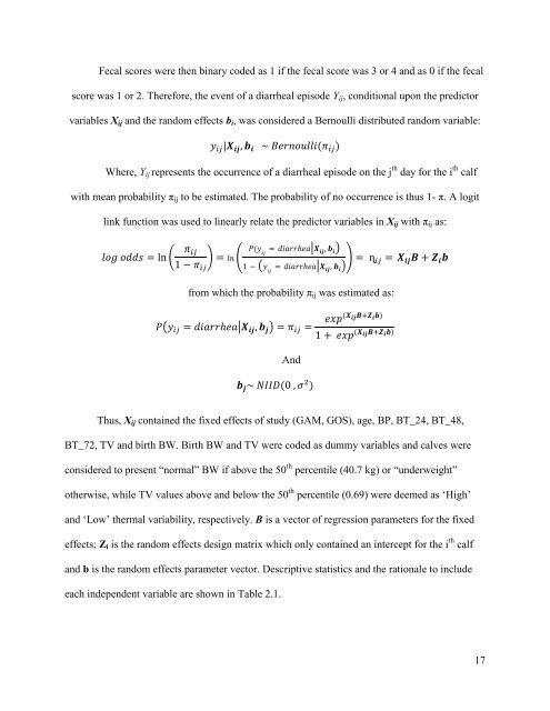
variables X ij and the random effects b i , was considered a Bernoulli distributed random variable:
Where, Y ij represents the occurrence of a diarrheal episode on the j th day for the i th calf
with mean probability π ij to be estimated. The probability of no occurrence is thus 1- π. A logit
link function was used to linearly relate the predictor variables in X ij with π ij as:
( ) (
| )
( | ) )
from which the probability π ij was estimated as:
( | )
And
Thus, X ij contained the fixed effects of study (GAM, GOS), age, BP, BT_24, BT_48,
BT_72, TV and birth BW. Birth BW and TV were coded as dummy variables and calves were
considered to present “normal” BW if above the 50 th percentile (40.7 kg) or “underweight”
otherwise, while TV values above and below the 50 th percentile (0.69) were deemed as ‘High’
and ‘Low’ thermal variability, respectively. B is a vector of regression parameters for the fixed
effects; Z i is the random effects design matrix which only contained an intercept for the i th calf
and b is the random effects parameter vector. Descriptive statistics and the rationale to include
each independent variable are shown in Table 2.1.
17