5128_Ch06_pp320-376

Section 6.1 Slope Fields and Euler’s Method 323
EXPLORATION 1
Seeing the Slopes
Figure 6.1 shows the general solution to the exact differential equation dydx cos x.
[–2π, 2π] by [–4, 4]
(a)
1. Since cos x 0 at odd multiples of p2 , we should “see” that dydx 0 at the
odd multiples of p2 in Figure 6.1. Is that true? How can you tell?
2. Algebraically, the y-coordinate does not affect the value of dydx cos x. Why not?
3. Does the graph show that the y-coordinate does not affect the value of dydx?
How can you tell?
4. According to the differential equation dydx cos x, what should be the slope of
the solution curves when x 0? Can you see this in the graph?
5. According to the differential equation dydx cos x, what should be the slope of
the solution curves when x p? Can you see this in the graph?
6. Since cos x is an even function, the slope at any point should be the same as the
slope at its reflection across the y-axis. Is this true? How can you tell?
Exploration 1 suggests the interesting possibility that we could have produced the family
of curves in Figure 6.1 without even solving the differential equation, simply by looking
carefully at slopes. That is exactly the idea behind slope fields.
Slope Fields
[–2π, 2π] by [–4, 4]
(b)
Suppose we want to produce Figure 6.1 without actually solving the differential equation
dydx cos x. Since the differential equation gives the slope at any point (x, y), we can use
that information to draw a small piece of the linearization at that point, which (thanks to
local linearity) approximates the solution curve that passes through that point. Repeating
that process at many points yields an approximation of Figure 6.1 called a slope field. Example
6 shows how this is done.
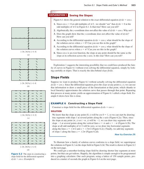
EXAMPLE 6
Constructing a Slope Field
Construct a slope field for the differential equation dydx cos x.
[–2π, 2π] by [–4, 4]
(c)
SOLUTION
We know that the slope at any point (0, y) will be cos 0 1, so we can start by drawing
tiny segments with slope 1 at several points along the y-axis (Figure 6.2a). Then, since
the slope at any point (p, y) or (p, y) will be 1, we can draw tiny segments with
slope 1 at several points along the vertical lines x p and x p (Figure 6.2b). The
slope at all odd multiples of p2 will be zero, so we draw tiny horizontal segments
along the lines x p2 and x 3p2 (Figure 6.2c). Finally, we add tiny segments
of slope 1 along the lines x 2p (Figure 6.2d).
Now try Exercise 29.
[–2π, 2π] by [–4, 4]
(d)
Figure 6.2 The steps in constructing a
slope field for the differential equation
dydx cos x. (Example 6)
To illustrate how a family of solution curves conforms to a slope field, we superimpose
the solutions in Figure 6.1 on the slope field in Figure 6.2d. The result is shown in Figure 6.3
on the next page.
We could get a smoother-looking slope field by drawing shorter line segments at more
points, but that can get tedious. Happily, the algorithm is simple enough to be programmed
into a graphing calculator. One such program, using a lattice of 150 sample points, produced
in a matter of seconds the graph in Figure 6.4 on the next page.