5128_Ch06_pp320-376

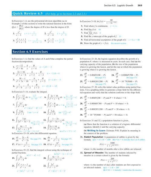
Section 6.5 Logistic Growth 369
Quick Review 6.5 (For help, go to Sections 2.2 and 2.3.)
In Exercises 1–4, use the polynomial division algorithm (as in
Example 2 of this section) to write the rational function in the form
R( x)
Q(x) , where the degree of R is less than the degree of D.
D ( x)
x
1. 2 1
x2
4
x 1 2. x 1
x 1
x
2
1
4 x
2
4
3. x 2
x 1
3
x2
1
x 2 x 2 4. x 3
5 5
x 2 x2
x
1 x
x2
1
60
In Exercises 5–10, let f (x) .
1 5e 0.1x
5. Find where f is continuous. (, )
6. Find lim f (x). 60
x→
7. Find lim f (x). 0
x→
8. Find the y-intercept of the graph of f. 10
9. Find all horizontal asymptotes of the graph of f. y 0, y 60
10. Draw the graph of y f (x). See answer section.
Section 6.5 Exercises
In Exercises 1–4, find the values of A and B that complete the partial
fraction decomposition.
12
1. x
x2
A 4x
x B
A 3, B 2
x 4
2x 16 A B
2. x
2
A 2, B 4
x 6 x 3 x 2
16 x A B
3. x 2
A 2, B 3
3x 10 x 2 x 5
3 A B
4. x 2
A 1/2, B 1/2
9 x 3 x 3
In Exercises 5–14, evaluate the integral.
12
⏐x⏐
3
2x 16
5. x
x2
dx ln
4x
(x 4) 2 C 6. x
2
dx ln ( x 2)
4
C
x 6 ( x 3)
2
2x 7. x
2
3 dx
8. x 2
6
4
x2
dx x ln 9 x 3
x 3
x 2 ln (x 2 4) 4 C
2 dx
3 dx
9. x
2
2 tan
1
1 x C 10. x
2
tan
9
1 x
3 C
7 dx
1 3x
11. 2x 2 12.
5x 3
3x
2
dx
x 3
5x 2
ln
2 x 1
C ln ⏐ x 2⏐
(3
8x 7
13. 2x
2
dx
14. 5 x 1) x 14
2 C
x 3
x
2 dx
7x
ln (1x 1⏐ 3 ⏐2x 3⏐) C
ln (x 2 ⏐x 7⏐ 3 ) C
In Exercises 15–18, solve the differential equation.
15. d y 2x
6
dx
x
2
See page 371. 16. d u 2
2x
dx
x 2 See page 371.
1
2
2t 17. F(x) x
3
See page 371. 18. G(t) 3
x
t
3
See page 371.
t
In Exercises 19–22, find the integral without using the technique of
partial fractions.
ln⏐x 2 ln⏐2x
4⏐ C
2 3x 1⏐ C
2x
4x 3
19. x
2
dx 20.
4
2x
2
dx
3x 1
21. x2 x 1
2x x
2 dx 22.
x
x
2
3 dx
1
x ln⏐x 2 x⏐ C
x 2 ln⏐x 2 1⏐ C
C
In Exercises 23–26, the logistic equation describes the growth of a
population P, where t is measured in years. In each case, find (a) the
carrying capacity of the population, (b) the size of the population
when it is growing the fastest, and (c) the rate at which the population
is growing when it is growing the fastest.
23. d P
0.006P(200 P) 24. d P
0.0008P(700 P)
dt
See page 371.
dt
See page 371.
25. d P
0.0002P(1200 P) 26. d P
10 5 P(5000 P)
dt
dt
See page 371.
See page 371.
In Exercises 27–30, solve the initial value problem using partial fractions.
Use a graphing utility to generate a slope field for the differential
equation and verify that the solution conforms to the slope field.
27. d P
0.006P(200 P) and P 8 when t 0.
dt
28. d P
0.0008P(700 P) and P 10 when t 0.
dt
29. d P
0.0002P(1200 P) and P 20 when t 0.
dt
30. d P
10 5 P(5000 P) and P 50 when t 0.
dt
In Exercises 31 and 32, a population function is given.
(a) Show that the function is a solution of a logistic differential
equation. Identify k and the carrying capacity.
(b) Writing to Learn Estimate P0. Explain its meaning in
the context of the problem.
31. Rabbit Population A population of rabbits is given by the
formula (a) k 0.7; M 1000 (b) P (0) 8; Initially there are 8 rabbits.
1000
Pt 1 e
4,
.80.7t
where t is the number of months after a few rabbits are released.
32. Spread of Measles The number of students infected by
measles in a certain school is given by the formula
200
Pt ,
1 e
5.3t
where t is the number of days after students are first exposed to
an infected student. (a) k 1; M 200
(b) P (0) 1; Initially 1 student has the measles.