5128_Ch06_pp320-376

More documents

Recommendations

Info

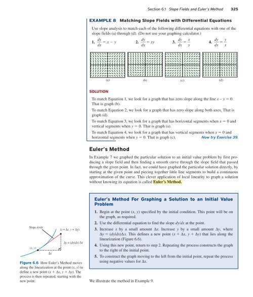
Section 6.1 Slope Fields and Euler’s Method 325 EXAMPLE 8 Matching Slope Fields with Differential Equations Use slope analysis to match each of the following differential equations with one of the slope fields (a) through (d). (Do not use your graphing calculator.) 1. d y x y 2. d y xy 3. d y x dx dx dx y 4. d y y dx x (a) (b) (c) (d) SOLUTION To match Equation 1, we look for a graph that has zero slope along the line x – y 0. That is graph (b). To match Equation 2, we look for a graph that has zero slope along both axes. That is graph (d). To match Equation 3, we look for a graph that has horizontal segments when x 0 and vertical segments when y 0. That is graph (a). To match Equation 4, we look for a graph that has vertical segments when x 0 and horizontal segments when y 0. That is graph (c). Now try Exercise 39. Euler’s Method In Example 7 we graphed the particular solution to an initial value problem by first producing a slope field and then finding a smooth curve through the slope field that passed through the given point. In fact, we could have graphed the particular solution directly, by starting at the given point and piecing together little line segments to build a continuous approximation of the curve. This clever application of local linearity to graph a solution without knowing its equation is called Euler’s Method. Slope dy/dx (x, y) Δx (x + Δx, y + Δy) Δy = (dy/dx) Δx Figure 6.6 How Euler’s Method moves along the linearization at the point (x, y) to define a new point (x Δx, y Δy). The process is then repeated, starting with the new point. Euler’s Method For Graphing a Solution to an Initial Value Problem 1. Begin at the point (x, y) specified by the initial condition. This point will be on the graph, as required. 2. Use the differential equation to find the slope dydx at the point. 3. Increase x by a small amount Δx. Increase y by a small amount Δy, where Δy (dy/dx)Δx. This defines a new point (x Δx, y Δy) that lies along the linearization (Figure 6.6). 4. Using this new point, return to step 2. Repeating the process constructs the graph to the right of the initial point. 5. To construct the graph moving to the left from the initial point, repeat the process using negative values for Δx. We illustrate the method in Example 9.
326 Chapter 6 Differential Equations and Mathematical Modeling 4 3 2 1 0 y 2 2.2 2.4 2.6 2.8 3 Figure 6.7 Euler’s Method is used to construct an approximate solution to an initial value problem between x 2 and x 3. (Example 9) x EXAMPLE 9 Applying Euler’s Method Let f be the function that satisfies the initial value problem in Example 6 (that is, dydx x y and f (2) 0). Use Euler’s method and increments of Δx 0.2 to approximate f (3). SOLUTION We use Euler’s Method to construct an approximation of the curve from x 2 to x 3, pasting together five small linearization segments (Figure 6.7). Each segment will extend from a point (x, y) to a point (x Δx, y Δy), where Δx 0.2 and Δy (dydx)Δx.The following table shows how we construct each new point from the previous one. (x, y) dydx x y Δx Δy (dydx)x (x Δx, y Δy) (2, 0) 2 0.2 0.4 (2.2, 0.4) (2.2, 0.4) 2.6 0.2 0.52 (2.4, 0.92) (2.4, 0.92) 3.32 0.2 0.664 (2.6, 1.584) (2.6, 1.584) 4.184 0.2 0.8368 (2.8, 2.4208) (2.8, 2.4208) 5.2208 0.2 1.04416 (3, 3.46496) Euler’s Method leads us to an approximation f (3) 3.46496, which we would more reasonably report as f (3) 3.465. Now try Exercise 41. You can see from Figure 6.7 that Euler’s Method leads to an underestimate when the curve is concave up, just as it will lead to an overestimate when the curve is concave down. You can also see that the error increases as the distance from the original point increases. In fact, the true value of f (3) is about 4.155, so the approximation error is about 16.6%. We could increase the accuracy by taking smaller increments; a reasonable option if we have a calculator program to do the work. For example, 100 increments of 0.01 give an estimate of 4.1144, cutting the error to about 1%. EXAMPLE 10 Moving Backward with Euler’s Method If dydx 2x y and if y 3 when x 2, use Euler’s Method with five equal steps to approximate y when x 1.5. SOLUTION Starting at x 2, we need five equal steps of Δx 0.1. (2, 3) (x, y) dy/dx 2x y Δx Δy (dydx)Δx (x Δx, y Δy) (2, 3) 1 0.1 0.1 (1.9, 2.9) (1.9, 2.9) 0.9 0.1 0.09 (1.8, 2.81) (1.8, 2.81) 0.79 0.1 0.079 (1.7, 2.731) (1.7, 2.731) 0.669 0.1 0.0669 (1.6, 2.6641) (1.6, 2.6641) 0.5359 0.1 0.05359 (1.5, 2.61051) [0, 4] by [0, 6] Figure 6.8 A grapher program using Euler’s Method and increments of 0.1 produced this approximation to the solution curve for the initial value problem in Example 10. The actual solution curve is shown in red. The value at x 1.5 is approximately 2.61. (The actual value is about 2.649, so the percentage error in this case is about 1.4%.) Now try Exercise 45. If we program a grapher to do the work of finding the points, Euler’s Method can be used to graph (approximately) the solution to an initial value problem without actually solving it. For example, a graphing calculator program starting with the initial value problem in Example 9 produced the graph in Figure 6.8 using increments of 0.1. The graph of the actual solution is shown in red. Notice that Euler’s Method does a better job of approximating the curve when the curve is nearly straight, as should be expected.
Page 1 and 2: Chapter6 Differential Equations and
Page 3 and 4: 322 Chapter 6 Differential Equation
Page 5: 324 Chapter 6 Differential Equation
Page 57:
376 Chapter 6 Differential Equation
show all

5128_Ch06_pp320-376

You also want an ePaper? Increase the reach of your titles

Delete template?

Save as template?