Sullivan Microsite TE SAMPLE

More documents

Recommendations

Info

Sullivan AP˙Sullivan˙Chapter01 October 8, 2016 17:4 Sullivan 128 Chapter 1 • Limits and Continuity Teaching Tip 1 Note that when finding the limit of x 2 as x approaches zero, the authors take a tabular and graphical approach. There is no algebraic manipulation that can be 1 performed to simplify the function , so a x 2 table or graph is the preferred method for this problem. Some students may prefer to create a table mentally when a written table is not required for the answer. For example, since zero cannot be substituted in this situation, the students may find it helpful to think, What does 1 divided by a really small positive number squared equal? Then they should think, What does 1 divided by a really small negative number squared equal? In both cases, the answer comes out to be an exceptionally large number, which grows increasingly large as x gets closer and closer to zero. Therefore. lim 1 =∞. x→0 2 x Teaching Tip It may be helpful for the students to keep these two limits in mind. They appear often as the students find one-sided limits and define vertical asymptotes. 1 lim =∞ x→ 0 + very small positive value 1 lim =−∞ x→0 − very small negative value Numerical examples help here as well: 1/0.1 = 10, 1/0.01 = 100, and so forth. For example, 1 = 1 1 1 = 0.1 10 1 = 0.01 100 1 = 0.001 1000 1 = 0.0001 10,000 y 4 1 Investigate Infinite Limits Consider the function f (x) = 1 . Table 11 lists values of f for selected numbers x that x 2 are close to 0 and Figure 48 shows the graph of f . Figure 48 f (x) = 1 x 2 As x approaches 0, the value of 1 x increases without bound. Since the value of 1 2 x is 2 not approaching a single real number, the limit of f (x) as x approaches 0 does not exist. TABLE 11 x approaches 0 x approaches 0 2 from the left −−−−−−−−−−−−−−−→ from the right ←−−−−−−−−−−−−−−−− x −0.01 −0.001 −0.0001 → 0 ← 0.0001 0.001 0.01 f (x) = 1 10,000 10 6 10 8 f (x) becomes unbounded 10 8 10 6 10,000 4 2 2 4 x x 2 x 0 y 4 2 2 4 2 4 4 Figure 49 f (x) = 1 x 2 x However, since the numbers are increasing without bound, we describe the behavior of the function near zero by writing 1 lim x→0 x =∞ 2 and say that f (x) = 1 has an infinite limit as x approaches 0. x 2 In other words, a function f has an infinite limit at c if f is defined everywhere in an open interval containing c, except possibly at c, and f (x) becomes unbounded when x is sufficiently close to c. ∗ EXAMPLE 1 1 1 Investigating lim and lim x→0 − x x→0 + x Consider the function f (x) = 1 . Table 12 shows values of f for selected numbers x x that are close to 0 and Figure 49 shows the graph of f . TABLE 12 x approaches 0 x approaches 0 from the left −−−−−−−−−−−−−−−−→ from the right ←−−−−−−−−−−−−−−−−− x −0.01 −0.001 −0.0001 → 0 ← 0.0001 0.001 0.01 0.1 f (x) = 1 x −100 −1000 −10,000 f (x) becomes unbounded 10,000 1000 100 10 Here as x gets closer to 0 from the right, the value of f (x) = 1 can be made as x large as we please. That is, 1 becomes unbounded in the positive direction. So, x Similarly, the notation 1 lim x→0 + x =∞ 1 lim x→0 − x = −∞ is used to indicate that 1 becomes unbounded in the negative direction as x approaches 0 x from the left. ■ ∗ A precise definition of an infinite limit is given in Section 1.6. 128 Chapter 1 • Limits and Continuity TE_Sullivan_Chapter01_PART II.indd 11 11/01/17 9:55 am
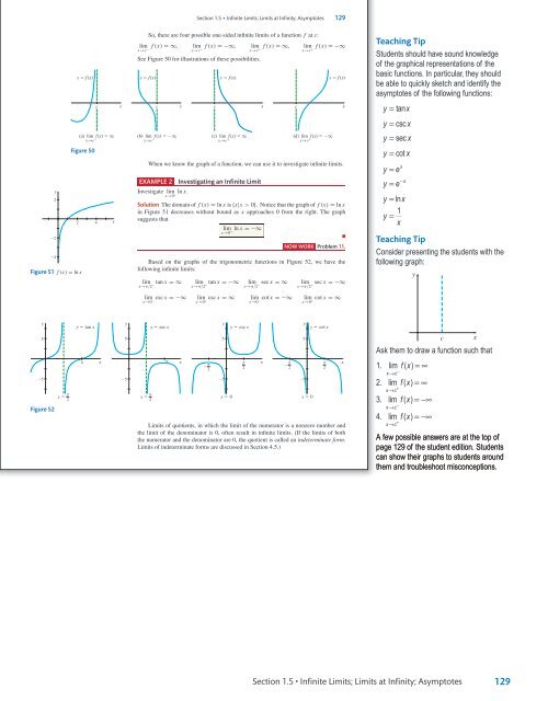
Sullivan AP˙Sullivan˙Chapter01 October 8, 2016 17:4 Section 1.5 • Infinite Limits; Limits at Infinity; Asymptotes 129 y 2 2 4 Figure 51 f (x) = ln x y f (x) lim x→c c x c x x→c x→c (a) lim f (x) ∞ (b) lim f(x) ∞ Figure 50 2 4 x So, there are four possible one-sided infinite limits of a function f at c: x→c x→c x→c + f (x) =∞, lim f (x) = −∞, lim f (x) =∞, lim − − + See Figure 50 for illustrations of these possibilities. y f (x) c y f (x) (c) lim f (x) ∞ x→c x c f (x) = −∞ (d) lim f (x) ∞ x→c y f (x) When we know the graph of a function, we can use it to investigate infinite limits. EXAMPLE 2 Investigate lim ln x. x→0 + Investigating an Infinite Limit Solution The domain of f (x) = ln x is {x|x > 0}. Notice that the graph of f (x) = ln x in Figure 51 decreases without bound as x approaches 0 from the right. The graph suggests that lim ln x = −∞ x→0 + ■ x NOW WORK Problem 11. Based on the graphs of the trigonometric functions in Figure 52, we have the following infinite limits: lim tan x =∞ lim x→π/2− lim csc x = −∞ lim x→0− tan x = −∞ lim x→π/2 + csc x =∞ lim x→0 + sec x =∞ lim x→π/2− cot x = −∞ lim x→0− sec x = −∞ x→π/2 + cot x =∞ x→0 + Teaching Tip Students should have sound knowledge of the graphical representations of the basic functions. In particular, they should be able to quickly sketch and identify the asymptotes of the following functions: y = tanx y = csc x y = sec x y = cot x y = y e x = e −x y = lnx 1 y = x Teaching Tip Consider presenting the students with the following graph: y y 5 5 π x 2 Figure 52 y y y y tan x y sec x y csc x y cot x π x 5 5 π x π 2 5 5 π x x 0 x 0 2 π 2 Limits of quotients, in which the limit of the numerator is a nonzero number and the limit of the denominator is 0, often result in infinite limits. (If the limits of both the numerator and the denominator are 0, the quotient is called an indeterminate form. Limits of indeterminate forms are discussed in Section 4.5.) x π 2 5 5 π 2 x Ask them to draw a function such that 1. lim fx ( ) =∞ x→c − 2. lim fx ( ) =∞ x→ c + 3. lim fx ( ) =−∞ x→c − 4. lim fx ( ) =−∞ x→ c + A few possible answers are at the top of page 129 of the student edition. Students can show their graphs to students around them and troubleshoot misconceptions. c x Section 1.5 • Infinite Limits; Limits at Infinity; Asymptotes 129 TE_Sullivan_Chapter01_PART II.indd 12 11/01/17 9:55 am
Page 2 and 3:
Chapter 1 Limits and Continuity Ove
Page 4 and 5:
Chapter 1: Resources TRM Teacher’
Page 6 and 7:
Sullivan AP˙Sullivan˙Chapter01 Oc
Page 8 and 9: Sullivan AP˙Sullivan˙Chapter01 Oc
Page 52 and 53: Teaching Tip Alternate Example Find
show all

Sullivan Microsite TE SAMPLE

Create successful ePaper yourself

Delete template?

Save as template?