Preferential Adsorption and Co-nonsolvency of ... - au one net

Received: November 26, 2010 

Revised: February 9, 2011 

Published: March 22, 2011 

ARTICLE 

pubs.acs.org/Macromolecules 

Preferential Adsorption and Co-nonsolvency of Thermoresponsive 

Polymers in Mixed Solvents of Water/Methanol 

Fumihiko Tanaka,* ,† Tsuyoshi Koga, † Hiroyuki Kojima, † Na Xue, ‡ and Franc-oise M. Winnik ‡ 

† 

Department of Polymer Chemistry, Graduate School of Engineering, Kyoto University, Katsura, Kyoto 615-8510, Japan 

‡ 

Department of Chemistry and Faculty of Pharmacy, University of Montreal, CP 6128, Succursale Centre Ville, Montreal QC, 

Canada H3C 3J7 

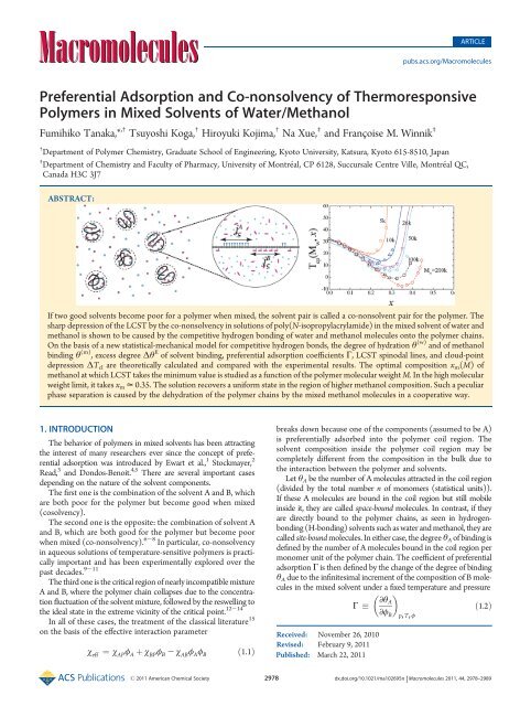
ABSTRACT: 

If two good solvents become poor for a polymer when mixed, the solvent pair is called a co-nonsolvent pair for the polymer. The 

sharp depression of the LCST by the co-nonsolvency in solutions of poly(N-isopropylacrylamide) in the mixed solvent of water and 

methanol is shown to be caused by the competitive hydrogen bonding of water and methanol molecules onto the polymer chains. 

On the basis of a new statistical-mechanical model for competitive hydrogen bonds, the degree of hydration θ (w) and of methanol 

binding θ (m) , excess degree Δθ E of solvent binding, preferential adsorption coefficients Γ, LCST spinodal lines, and cloud-point 

depression ΔTcl are theoretically calculated and compared with the experimental results. The optimal composition xm(M) of 

methanol at which LCST takes the minimum value is studied as a function of the polymer molecular weight M. In the high molecular 

weight limit, it takes xm = 0.35. The solution recovers a uniform state in the region of higher methanol composition. Such a peculiar 

phase separation is caused by the dehydration of the polymer chains by the mixed methanol molecules in a cooperative way. 

1. INTRODUCTION 

The behavior of polymers in mixed solvents has been attracting 

the interest of many researchers ever since the concept of preferential 

adsorption was introduced by Ewart et al., 1 Stockmayer, 2 

Read, 3 and Dondos-Benoit. 4,5 There are several important cases 

depending on the nature of the solvent components. 

The first one is the combination of the solvent A and B, which 

are both poor for the polymer but become good when mixed 

(cosolvency). 

The second one is the opposite: the combination of solvent A 

and B, which are both good for the polymer but become poor 

when mixed (co-nonsolvency). 6-8 In particular, co-nonsolvency 

in aqueous solutions of temperature-sensitive polymers is practically 

important and has been experimentally explored over the 

past decades. 9-11 

The third one is the critical region of nearly incompatible mixture 

A and B, where the polymer chain collapses due to the concentration 

fluctuation of the solvent mixture, followed by the reswelling to 

theidealstateintheextremevicinityofthecriticalpoint. 12-14 

In all of these cases, the treatment of the classical literature 15 

on the basis of the effective interaction parameter 

χ eff ¼ χ AP φ A þ χ BP φ B - χ AB φ Aφ B 

ð1.1Þ 

breaks down because one of the components (assumed to be A) 

is preferentially adsorbed into the polymer coil region. The 

solvent composition inside the polymer coil region may be 

completely different from the composition in the bulk due to 

the interaction between the polymer and solvents. 

Let θA be the number of A molecules attracted in the coil region 

(divided by the total number n of monomers (statistical units)). 

If these A molecules are bound in the coil region but still mobile 

inside it, they are called space-bound molecules. In contrast, if they 

are directly bound to the polymer chains, as seen in hydrogenbonding 

(H-bonding) solvents such as water and methanol, they are 

called site-bound molecules. In either case, the degree θA of binding is 

defined by the number of A molecules bound in the coil region per 

monomer unit of the polymer chain. The coefficient of preferential 

adsorption Γ is then defined by the change of the degree of binding 

θA due to the infinitesimal increment of the composition of B molecules 

in the mixed solvent under a fixed temperature and pressure 

r 2011 American Chemical Society 2978 dx.doi.org/10.1021/ma102695n | Macromolecules 2011, 44, 2978–2989 

Γ 

∂θA 

∂φ B p, T, φ 

ð1.2Þ

Macromolecules ARTICLE 

where φ is the volume fraction of the polymer and φB the volume 

fraction of the second solvent. A small change in φ B may cause a 

large effect on the fraction θA of the adsorbed molecules. 

The preferential adsorption coefficient was first introduced by 

Ewart et al. 1 by the definition R -(dm B/dm) p,T,μB to determine 

the polymer molecular weight in mixed solvents by light 

scattering, where m and mA, mB are the molarity of the polymer, 

the primary and secondary solvent and μB is the chemical 

potential of the second solvent. Later, a more general theory of 

concentration fluctuations in relation to light scattering intensity 

in multicomponent systems was developed by Stockmayer, 2 in 

which the adsorption coefficient was shown to be proportional to 

(∂μB/∂m)m B /(∂μB/∂mB)m. In order to see the sensitivity of the 

bound A molecules to mixed B solvent more directly, we study 

here the preferential adsorption by introducing the coefficient Γ 

under a fixed finite polymer concentration, which is related to the 

reduction of the bound A molecules to the infinitesimal increment 

of the B composition in the mixed solvent. This coefficient 

may be applied to both space-bound case and site-bound case 

equally well. Condensation of counterions near the polymer 

chains fall on the former category. The bound molecules, or ions, 

move with the polyelectrolyte polymer chains, so that the mixing 

entropy is substantially reduced. 

The statistical-thermodynamics of preferential adsorption in 

mixed solvents was attempted by Yamamoto et al. 16 by introducing 

a coating monolayer into the conventional Flory-Huggins 

theory of polymer solutions within quasi-chemical approximation. 

The idea was later applied to the chain conformation in 

mixed solvents. 17 Though the idea hit the central concept of 

preferential adsorption, this theory unfortunately remained too 

complicate to reach specific results regarding the problems 

described above. 

The problem of the chain dimensions in critical solvent mixtures 

was first studied by de Gennes 12 on the basis of preferential 

adsorption for the case where A and B are both good and for the 

case where A is good but B is poor. It was found that the polymer 

chain collapses in the critical region due to the attractive 

interaction between the polymer segments. 12 The source of this 

effect is indirect long-range interaction between monomers; one 

monomer creates a cloud of preferential solvation in its vicinity, 

and a second monomer is then attracted by this cloud. The 

interaction range is decided by the correlation length ξ of the 

A/B mixture, which can be large near the critical point. The result 

was later refined by including the shift of the critical temperature 

inside the coil region when the polymer collapses. 13 The drastic 

shift of the coexistence line of A/B solvent mixture near the 

critical point induced by adding small quantity of polymers was 

experimentally confirmed by Dondos and Izumi. 14 There have 

been recently renewed interest in the problem of polymer 

conformation in critical solvent mixtures. For instance, Grabowski 

et al. 18 experimentally confirmed contraction and reswelling 

of poly(acrylic acid)in a critical 2,6-lutidine/water mixture by the 

measurement of the diffusion constant. Refinement of the theory 

by field theoretical calculation of the polymer dimensions in 

critical solvent mixtures was also attempted. 19 

Polymers in aqueous media in contrast exhibit a more 

dramatic behavior due to the direct H-bonding of water molecules 

when the second solvent is mixed. For instance, poly(Nisopropylacrylamide) 

(PNIPAM) exhibits peculiar conformational 

changes in water upon mixing of a second water-miscible 

solvent such as methanol, tetrahydrofuran, or dioxane. Although 

the second solvent is a good solvent for the polymer, the polymer 

chain collapses in certain compositions of the mixed solvent, 

followed by the reswelling under majority of the second solvent. 20 

The tendency for phase separation is also strongly enhanced 

by the presence of the second solvent. For instance, the LCST of 

aqueous PNIPAM solutions shifts to lower temperature when 

methanol is added. 9-11 The temperature drop is the largest, from 

31.5 °C down to -7 °C, for the specific molar fraction xm = 0.35 

of methanol. This enhanced phase separation in mixed good solvents 

is known as co-nonsolvency. 9 Cross-linked PNIPAM gels are 

also known to collapse sharply in water in the presence of 

methanol, at around xm = 0.3, and gradually recover their swollen 

state with increasing methanol content. 21-23 

There have been efforts to understand co-nonsolvency by the 

combination of three χ-parameters 9 and also by the formation of 

stoichiometric compounds between the solvent molecules. 20 

Without considering direct hydrogen bonds between polymer 

and solvents, however, it is difficult to explain sharp LCST behavior 

and sensitivity to the molecular weight of the polymers. 

We recently showed that, in solutions of PNIPAM in a mixed 

solvent of water and methanol, the competition in forming 

PNIPAM-water (p-w) H-bonds and PNIPAM-methanol 

(p-m) H-bonds (competitive adsorption) results in co-nonsolvency. 

24,25 In such a case, the second solvent molecules are also 

site-bound. The bound methanol molecules block the formation 

of continuous trains of bound water molecules caused by the 

cooperativity of hydration. Small difference in the composition of 

the mixed solvent is greatly amplified, and, as a result, the 

composition of the bound molecules along the chain deviates 

substantially from that in the bulk (nonlinear amplification). The 

total coverage θ = θA þ θB of the chain by bound molecules 

exhibits a minimum at the composition where the competition is 

strongest; hence, the chain collapses around this composition by 

hydrophobic aggregation of the dehydrated chain segments. 

In this paper, we apply our model of cooperative hydration to 

the preferential adsorption and phase separation of PNIPAM in a 

mixed solvent of water and methanol. We calculate the fraction of 

bound water, the preferential adsorption coefficient, spinodal line, 

etc., as a function of the composition of the mixed solvent and 

report that the phase transition becomes sharper with increasing 

cooperativitiy, and hence the effect of co-nonsolvency is enhanced. 

2. THE MODEL OF PREFERENTIAL ADSORPTION IN 

HYDROGEN-BONDING MIXED SOLVENTS 

The model we consider is a polymer solution in which the 

number N of polymer chains with degree of polymerization 

(referred to as DP) n are dissolved in the number NA of A solvent 

molecules and the number NB of B solvent molecules. The 

polymer chains are H-bonded with both solvents A and B 

(Figure 1). We are specifically interested in PNIPAM dissolved 

in water (w) as the primary solvent A, and methanol (m) as the 

secondary solvent B. But the model is general enough to be 

applied to other polymer solutions with both site- and spacebound 

solvents. 

The solvents A and B are assumed to be mutually miscible, and 

they are capable of forming H-bonds with the polymer chains 

(site-binding case). Therefore, there is a competition in forming 

p-A and p-B H-bonds. 

We are based on the lattice-theoretical picture of polymer 

solutions and divide the system volume V into cells of size a, each 

of which can accommodate a statistical repeat unit of the 

polymer. The volume of the solvent molecule is assumed to be 

2979 dx.doi.org/10.1021/ma102695n |Macromolecules 2011, 44, 2978–2989


Figure 1. Model solution of hydrogen-bonded polymers in a mixed 

solvent. Both solvents A and B are assumed to be capable of forming 

hydrogen bonds with the polymers, so that there is a competition in 

forming p-A and p-B hydrogen bonds. 

nA for A and nB for B in the unit of the cell volume. We assume 

incompressibility of the solution, so that we have Ω = nN þ 

n AN A þ n BN B,whereΩ V/a 3 is the total number of cells. 

To describe the H-bonds of A and B with the polymer chains, 

let (l, m) be the type of the polymer chains which carry the 

number l of bound A molecules and m of bound B molecules and 

let Nl,m be the number of polymers of the type (l, m) in the 

solution. The total number of A molecules on a chain is ∑lNl,m, 

and B molecules is ∑mNl,m. Let NfA be the number of free A 

molecules, and let N fB be that of free B molecules. 

We then have the material conservation laws 

and 

N ¼ X 

Nl, m 

l, m 

NA ¼ NfA þ X 

NB ¼ NfB þ X 

lNl, m 

l, m 

mNl, m 

l, m 

Ω ¼ X 

ðn þ nAl þ nBmÞNl, m þ nANfA þ nBNfB 

l, m 

The free energy we consider is 

βΔF ¼ X 

Nl, m ln φl, mþNfA ln φfA þ NfB ln φfB l, m 

ð2.1aÞ 

ð2.1bÞ 

ð2.1cÞ 

ð2.2Þ 

þ X 

Δl, mNl, m þ ΩgðfφgÞ ð2.3Þ 

l, m 

where β 1/kBT, and 

φl, m ðnþnAl þ nBmÞNl, m=Ω ð2.4Þ 

is the volume fraction of the (l, m) polymers, and 

φf R nRNfa=Ω ðR ¼ A, BÞ ð2.5Þ 

are the volume fractions of the free solvent molecules. The 

number density of the complex molecules of the type (l, m) is 

νl, m ¼ Nl, m=Ω ð2.6Þ 

The free energy 

Δl, m βΔAl, m ð2.7Þ 

for the formation of a complex of the type (l, m) depends on the 

details of the H-bonds, which will be specified when we calculate 

the solution properties. 

The molecular interaction is included in the last term of eq 2.3 

in the form 

gðfφgÞ ðχAφA þ χBφBÞφ þ χABφAφB ð2.8Þ 

where χA, χB, and χAB are Flory’s interaction parameters between 

polymer and A-solvent (p/A), polymer and B-solvent (p/B), and 

A-solvent and B-solvent (A/B). They are based on the van der 

Waals interaction in the background and functions of the temperature 

only. (We do not assume ternary interaction term χTφφAφB in 

the free energy because its molecular origin is not clear.) 

By differentiation with respect to Nl,m, NfA, and NfB, wefind 

the chemical potentials 

βΔμl, m 

n þ nAl þ nBm ¼ 1 þ Δl, m þ ln φl, m 

n þ nAl þ nBm - νS þ gl, m ð2.9Þ 

for the polymer of (l, m) type, and 

βΔμfA =nA ¼ð1þln φfAÞ=nA - ν S þ gfA ð2.10aÞ 

βΔμ fB =nB ¼ð1 þ ln φ fBÞ=nB - ν S þ gfB 

for the free solvent molecules, where 

v S 

X 

vl, mþ φfA þ 

nA 

φfB nB 

l, m 

ð2.10bÞ 

ð2.11Þ 

is the total number of translational degree of freedom in the 

solution, and 

gfA - g þ χAφ þ χABφB ð2.12aÞ 

gfB - g þ χ B φ þ χ AB φ A ð2.12bÞ 

have appeared from the interaction terms. Also, we have 

gl, m 

ng0, 0 þ nAlgfA þ nBmgfB 

n þ nAl þ nBm 

ð2.13Þ 

for the (l, m) complexes, where 

g0, 0 - g þ χAφA þ χBφB ð2.14Þ 

By imposing the association equilibrium conditions 

Δμl, m ¼ Δμ0, 0 þ lΔμfA þ mΔμfB ð2.15Þ 

we find 

l m 

φl, m ¼ Kl, mφ0, 0φfA φfB ð2.16Þ 

where 

Kl, m ¼ expðl þ m - Δl, mÞ ð2.17Þ 

is the equilibrium constant. Let us write as x φ0,0 and yR φfR (R = A, B) for the bare polymer chains and the free solvent 

molecules. We then have 

φ ¼ nxpðyA, yBÞ ð2.18aÞ 

φA ¼ yA þ nAφθAðyA, yBÞ ð2.18bÞ 

φB ¼ yB þ nBφθBðyA, yBÞ ð2.18cÞ 

by the material conservation laws (2.1a) to (2.1c), where the 

function p(yA,yB) isdefined by 

pðyA, yBÞ 

X 

bl, my l AymB ð2.19Þ 

2980 dx.doi.org/10.1021/ma102695n |Macromolecules 2011, 44, 2978–2989 

l, m


(bl,m Kl,m/(n þ nAl þ nBm)). This function is called binding 

polynomial in the literature. It is equivalent to the grand partition 

function of a H-bonding chain in the mixed solvent. 

The degree of binding for each component is defined by the 

average number of bound molecules per binding site on the 

polymer chain and derived from the binding polynomial by 

differentiation 

θRðyA, yBÞ 

1 ∂ ln p 

n ∂ ln yR 

ðR ¼ A, BÞ ð2.20Þ 

In summary, we have found 

βΔμ0, 0 ¼ 1 þ ln x - nv S þ ng0, 0 ð2.21aÞ 

βΔμ fA ¼ 1 þ ln yA - nAv S þ nAgfA 

βΔμ fB ¼ 1 þ ln yB - nBv S þ nBgfB 

ð2.21bÞ 

ð2.21cÞ 

with 

v S ¼ φ=n þ yA=nA þ yB=nB ð2.22Þ 

Substituting the equilibrium distribution function (2.16) back 

into the original free energy, we find 

βΔF=Ω ¼ F FH þ F AS ð2.23Þ 

where 

F FH ¼ φ 

n ln φ þ φA ln φA þ 

nA 

φB ln φB þ gðfφgÞ ð2.24Þ 

nB 

is the conventional Flory-Huggins free energy, and 

F AS ¼ φ x 

ln 

n φ þ φA ln 

nA 

yA 

þ 

φA φB ln 

nB 

yB 

þðθA þ θBÞφ 

φB ð2.25Þ 

is the free energy due to the molecular association. 

3. PREFERENTIAL ADSORPTION BY POLYMERS IN 

MIXED SOLVENTS 

The total degree of binding is 

θ θA þ θB ð3.1Þ 

If there is no interaction between the bound molecules, the total 

is given by the simple mixing law 

ð3.2Þ 

where θR° is the degree of binding in each pure solvent, and 

xR NR=ðNA þ NBÞ ðR¼A, BÞ ð3.3Þ 

are the mole fractions of the solvent. The excess binding is then 

defined by 

Δθ E 

θ° θ ° 

A xA þ θ ° 

B xB 

θ - θ° ¼ θA - θ ° 

A xA þ θB - θ ° 

B xB 

ð3.4Þ 

For cosolvency, the excess is positive, while for co-nonsolvency 

it is negative. There is a possibility that the excess binding 

changes its sign at a certain composition of the mixed solvent. 

The mole fraction of the bound molecules at such a particular 

concentration takes exactly the same value as the mole fraction of 

the solvent in the bulk outside the coil region. Such a particular 

point is called azeotropic binding. 26 

In what follows we focus on co-nonsolvency, and derive Gibbs 

matrix for the study of phase separation. As for the composition 

of the solvent mixture, we use its volume fraction 

vR nRNR=ðnANA þ nBNBÞ ðR¼A, BÞ ð3.5Þ 

as well as the mole fraction. We then have 

φA ¼ð1-φÞvA, φB ¼ð1-φÞvB ð3.6Þ 

We regard the volume fraction vB of the second solvent as the 

controlling parameter, and write it as vB ξ. We then have vA =1 

- ξ. 

3.1. Transition Matrix. Let us first relate the variation of the 

volume fraction yA and yB of the free solvents by the variation of 

the independent variable φA and φB (solvent composition) which 

are controlled variables in the experiments. We first define a 

matrix JR,β by the equation 

d ln yR ¼ X 

JR, βdφβ ð3.7Þ 

Or, in the matrix form 

2 3 

dlnyA 

4 5 ¼ 

dlnyB 

JA, 

2 3 

A 

4 

JB, A 

JA, B 

5 

JB, B 

dφ 2 3 

A 

4 5 

dφB ð3.8Þ 

By taking the derivatives of the material conservation laws 

(2.18a) to (2.18c), we have 

p dx þ φðθA dlnyA þ θB dlnyBÞ ¼ - ðdφA þ dφBÞ=n ðyA þ nAφθAKA, AÞ dlnyA þ nAφ AθAKA, B dlnyB 

2981 dx.doi.org/10.1021/ma102695n |Macromolecules 2011, 44, 2978–2989 

β 

¼ð1 þ nAθAÞ dφ A þ nAθA dφ B 

nBφθBKB, A dlnyB þðyB þ nBφθBKB, BÞ dlnyB 

¼ nBθB dφA þð1þ nBθBÞ dφB where the matrix KR,β is defined by 

∂ ln θR 

KR, β 

∂ ln yβ 

Solving these equations for d lnyR, we find 

JA, A ¼fð1-φB- yAÞ½yB þðφB - yBÞKB, BŠ 

- ðφA - yAÞðφB - yBÞKA, Bg=φΦ 

ð3.9Þ 

ð3.10Þ 

JA, B ¼ðφ A - yAÞ½yB - φKA, B þðφ B - yBÞðKB, B - KA, BÞŠ=φΦ 

JB, A ¼ðφ B - yBÞ½yA - φKB, A þðφ A - yAÞðKA, A - KB, AÞŠ=φΦ 

JB, B ¼fð1-φA- yBÞ½yA þðφA - yAÞKA, AŠ 

- ðφB - yBÞðφA - yAÞKB, Ag=φΦ ð3.11Þ 

where 

ΦðyA, yBÞ yAyB þðφA - yAÞyBKA, A þðφB - yBÞyAKB, B 

þðφA - yAÞðφB - yBÞK ð3.12Þ 


K KA, AKB, B - KA, BKB, A ð3.13Þ 

is the determinant of the matrix ^K.


3.2. Preferential Adsorption Coefficients. The preferential 

adsorption coefficient ΓR,β is defined by the change d ln θR of the 

adsorbed R-component by an infinitesimal increment dφβ of the 

β-component solvent. By multiplication of K matrix to the 

transition J matrix, we find 

2 3 

dlnθA 

4 5 ¼ 

dlnθB 

KA, 

2 3 

A KA, B 

4 5 

KB, A KB, B 

JA, 

2 3 

A JA, B 

4 5 

JB, A JB, B 

dφ 2 3 

A 

4 5 

dφB ¼ ΓA, 

" # " # 

A ΓA, B dφA 

ð3.14Þ 

ΓB, A ΓB, B dφB where 

ΓA, A ¼fð1-φB- yAÞ½yBKA, A þðφB - yBÞKŠ 

þðφB - yBÞyAKA, Bg=φΦ 

ΓA, B ¼fð1 - φ A - yBÞyAKA, B þðφ A - yAÞyBKA, A 

þðφ A - yAÞðφ B - yBÞKg=φΦ 

ΓB, A ¼fð1 - φ B - yAÞyBKB, A þðφ B - yBÞyAKB, B 

þðφ A - yAÞðφ B - yBÞKg=φΦ 

ΓB, B ¼fð1-φA- yBÞ½yAKB, B þðφA - yAÞKŠ 

þðφA - yAÞyBKB, Ag=φΦ ð3.15Þ 

If the volume fraction φ of the polymer is fixed, dφ A and dφ B 

are not independent, but related by 

dφ A ¼ - ð1 - φÞdξ ð3.16aÞ 

dφB ¼ð1-φÞdξ ð3.16bÞ 

and hence the preferential adsorption coefficient is 

∂θA 

Γ 

∂ξ 

ð1 - φÞθA 

¼ 

φΦðyA, yBÞ ½ð - yBKA, A þ yAKA, BÞφ - ðφB - yBÞφKŠ 

Here yA and yB are the solutions of the coupled equations 

ð3.17Þ 

yA þ nAφθAðyA, yBÞ ¼ð1 - φÞð1 - ξÞ ð3.18aÞ 

yB þ nBφθBðyA, yBÞ ¼ð1 - φÞξ ð3.18bÞ 

4. PHASE SEPARATION IN MIXED SOLVENTS 

Although we are ready to find the binodals by using the 

chemical potentials, we are involved in many technical difficulties 

for numerical calculations of three-component systems, in particular 

in the presence of the cooperativity in the H-binding. 

Therefore, we attempt to find spinodal lines only by the calculation 

of Gibbs matrix. 

4.1. Construction of the Gibbs Matrix. In tertiary systems, 

two of the three chemical potentials are independent due to the 

Gibbs-D€uhem relation. Here we use the chemical potentials 

of the free solvent molecules. The Gibbs matrix is then defined by 

GR, β 

∂Δμ f R 

∂φ β 

Because we have 

dv S 

vA dφA þ vB dφB for the variation of ν S , where 

and also 

vA 

vB 

- 1 

n 

- 1 

n 

þ yA 

nA 

þ yA 

nA 

JA, A þ yB 

JA, B þ yB 

JB, A 

nB 

JB, B 

nB 

" # 

dgfA 

¼ 

dgfB 

gA, 

" # " # 

A gA, B dφA 

gB, A gB, B dφB ð4.1Þ 

ð4.2Þ 

ð4.3aÞ 

ð4.3bÞ 

ð4.4Þ 

for the variation of the interaction, we find 

" # 

dΔμfA ¼ 

dΔμfB " # " # 

JA, A - nAvA þ nAgA, A JA, B - nAvB þ nAgA, B dφA 

JB, A - nBvA þ nBgB, A JB, B - nBvB þ nBgB, B dφB ð4.5Þ 

for the variation of the chemical potentials, where 

gA, A - 2χAφ - ðχA - χB þ χABÞφB ð4.6aÞ 

gA, B - χ B ðφ - φ BÞ - ðχ A - χ AB Þð1 - φ AÞ ð4.6bÞ 

gB, A - χ A ðφ - φ AÞ - ðχ B - χ AB Þð1 - φ BÞ ð4.6cÞ 

gB, B - 2χ B φ þðχ A - χ B - χ AB Þφ A ð4.6dÞ 

The Gibbs matrix is 

^G ¼ JA, 

" 

A - nAvA þ nAgA, A 

JB, A - nBvA þ nBgB, A 

# 

JA, B - nAvB þ nAgA, B 

JB, B - nBvB þ nBgB, B 

ð4.7Þ 

4.2. Spinodal Condition. The spinodal condition is given by 

|^G| = 0. After lengthy calculation, we finally find 

- nnAnB~χφΦ - 2nAnBχABðΦ þ nΨÞ - 2nðχAΦA þ χBΦBÞ þ ΨA þ ΨB þ nð1 þ nAθA þ nBθBÞ 2 φ ¼ 0 ð4.8Þ 

where Φ is defined by eq 3.12. The rests are 

Ψ yBθAðφA - yAÞþyAθBðφB - yBÞ 

þ 1 

2 φ2ðθAKA, B þ θBKB, AÞþðφA - yAÞðφB - yBÞ½θAðKB, B - KA, BÞ 


þ θBðKA, A - KB, AÞŠ ð4.9Þ 

ΨA nAyA þðφ A - yAÞðnAKA, A þ nBKA, BÞ ð4.10aÞ 

ΨB nByB þðφ B - yBÞðnBKB, B þ nAKB, AÞ ð4.10bÞ 



ΦA 

ΦB 

ΨAφ þðφA - yAÞðφB - yBÞ½nAðKB, A - KA, AÞ 

- nBðKA, B - KB, BÞŠ ð4.10cÞ 

ΨBφ þðφA - yAÞðφB - yBÞ½nBðKA, B - KB, BÞ 

- nAðKB, A - KA, AÞŠ ð4.10dÞ 

The effective interaction parameter χ~ is defined by 

~χ χ A 2 þ χB 2 þ χAB 2 - 2χA χ B - 2χ A χ AB - 2χ B χ AB ð4.11Þ 

5. RANDOM HYDRATION 

For random hydration, the coefficient bl,m in eq 2.19 is 

proportional to the number of different ways to place l of A 

molecules and m of B molecules on the total cites n, and hence bl,m 

∼ n!/l!m!(n - l - m)!. Let λR(T) exp(-fR/kBT) bethe 

association constant of the H-bonding of R molecule. (f R is the 

binding free energy of a single H-bond.) We then find as usual 

Langmuir type competitive adsorption of molecules. The binding 

polynomial is 

where 

We then have 

pðyA, yBÞ ¼t -n 

ð5.1Þ 

t 1=ð1 þ λAyA þ λByBÞ ð5.2Þ 

θA ¼ λAyAt ð5.3aÞ 

θB ¼ λByBt ð5.3bÞ 

From the materials conservation law (2.1a) to (2.1c), the volume 

fractions of the free solvents are written as 

yA ¼ φ A=ð1 þ nAλAφtÞ ð5.4aÞ 

yB ¼ φA=ð1 þ nBλBφtÞ ð5.4bÞ 

Substituting into eq 5.2, we find that the equation to decide t as a 

function of the total volume fractions of the solvents is given by 

nAnBλAλBφ 2 t 3 þ½λAλBðnBφA þ nAφBÞþnAλA þ nBλB 

- nAnBλAλBφŠφt 2 þðλAφA þ λBφBÞt - 1 ¼ 0 

The ^K matrix takes the form 

ð5.5Þ 

^K ¼ 1 - θA, 

" 

-θA, 

# 

-θB 

1-θB ð5.6Þ 

Its determinant is 

K ¼ 1 - θ ð5.7Þ 

where θ = θAþ θB is the total degree of binding, and Φ reduces to 

Φ ¼ φAφBð1 - θÞþyAθAφB þ yBθBφA ð5.8Þ 

The preferential adsorption coefficient is 

ð1 - φÞθA 

Γ ¼ - 

φΦ f½yBð1 - θAÞþyAθBŠφ 

þðφB - yBÞð1 þ φA - φB - 2yAÞð1 - θÞg ð5.9Þ 

The spinodal condition is given by eq 4.8, where we have 

specifically 

Ψ ¼ φ Aφ B - Φ ð5.10aÞ 

ΨA ¼ nAyA þ½nAð1 - θAÞ - nBθBŠðφ A - yAÞ ð5.10bÞ 

ΨB ¼ nByB þ½nBð1 - θBÞ - nAθAŠðφ B - yBÞ ð5.10cÞ 

ΦA ¼½nAφA- ðnAθA þ nBθBÞðφA - yAÞŠφ 

- ðnA - nBÞðφA - yAÞðφB - yBÞ ð5.10dÞ 

ΦB ¼½nBφB- ðnAθA þ nBθBÞðφB - yBÞŠφ 

- ðnB - nAÞðφB - yBÞðφA - yAÞ ð5.10eÞ 

Obviously, there is no excess binding Δθ E =0. 

For numerical calculation of the phase diagrams, we fix the 

necessary parameters in the following way. We first assume the 

conventional Shultz-Flory form 

nAχ A ðTÞ ¼nBχ B ðTÞ ¼1=2 - ψτ ð5.11Þ 

for the χ-parameters, 27 where τ =1- Θ 0/T is the reduced 

temperature deviation measured from the reference theta temperature 

Θ0 satisfying χ(Θ0) = 1/2, and ψ is a material 

parameter of order unity. At the temperature Θ 0, the second 

virial coefficient of a hypothetical Flory-Huggins solution without 

hydrogen-bonding interaction vanishes. The reference temperature 

Θ0 is not the true theta temperature Θ at which the 

second virial coefficient of the osmotic pressure vanishes. The 

latter lies far below Θ0. As for A/B interaction, we assume the 

athermal mixture χAB = 0 because the mixed solvent is completely 

miscible. 

The association constant is then expressed as λA(T) = λA0 

exp(|ε|/kBT)=λA0 exp[γA (1- τ)], where λA0 gives the entropy 

part of the binding free energy, and γ A 

|ε|/k BΘ 0 gives the 

binding energy of a water molecule measured relative to the 

thermal energy at the reference theta temperature. Throughout 

the present numerical calculation, we fix ψ at ψ = 1.0, and other 

parameters are n=100, nA = nB =1,λA0 = 0.002, γA = 3.5, and 

σA = 1.0. 

Figure 2a shows how the phase diagram shifts by mixing the 

fictitious second solvent, which is assumed to be symmetric to 

water, but with slightly different H-bonding amplitude λB0 = 

0.003 . The volume fraction of the second solvent is varied from 

curve to curve. The miscibility loop monotonically shrinks with 

the volume fraction ξ. The bottom part of the miscibility loop 

corresponds to the LCST phase separation. 

Figure 2b shows the spinodal temperature plotted against the 

volume fraction ξ of the second solvent. The amplitude λB0 of the 

H-bond of the second solvent is varied from curve to curve. For 

small values of λB0, the LCST decreases (the miscibility gap 

expands) with the composition of the second solvent, while for 

large values of λB0, it goes up (the miscibility gap shrinks). 

Figure 3a shows the binding isotherms of the completely 

symmetric solvent pair A and B at the polymer concentration φ = 

0.1 plotted against the solvent composition. The temperature is 

fixed at τ = -1.0. The amplitude of the H-bond is fixed at λA0 = 

λ B0 = 0.002. Because the adsorption takes place independently, 

θA decreases in proportion to the composition (Raoult’s law), 

while θB increases in proportion to the composition (Henry’s 

law). The composition of the adsorbed molecules is the same as 



Figure 2. (a) Phase diagrams on the (φ,τ) plane for random binding. The solvent composition ξ is changed from curve to curve. (b) Shift of LCST line 

by mixing the second solvent for the polymer volume fraction φ = 0.1. The strength λB0 is changed, while γ = 3.5 is fixed. 

Figure 3. (a) Binding isotherm for random adsorption. The degree of binding for each solvent component and the total degree of binding are plotted 

against the solvent composition ξ in the symmetric case nA = nB = 1 and λA(T) =λB(T) = 0.002. (b) Preferential adsorption coefficient Γ plotted 

against ξ. 

that in the bulk. The total degree of adsorption θ = θ A þ θ B is 

therefore independent of the solvent composition. 

Figure 3b shows the preferential adsorption coefficient plotted 

against the solvent composition. It is negative and independent 

of the solvent composition. It gives the initial slope of θA in 

Figure 3a if we put ξ =0. 

6. COOPERATIVE HYDRATION 

If there is attractive interaction between the adjacent bound 

molecules of the same species, H-bonding is not random but 

cooperative. Each chain carries continuous H-bonding sequences 

of A and of B (Figure 1). Let j ζ A be the number of the 

A-sequences that consist of a number ζ of contiguous bound A 

molecules, and let jζ B be that of the B-sequences. The H-bonded 

A A B 

{j1 ,j2 ,...} and j 

state of a chain is specified by the indices j A 

{j1 B ,j2 B ,...}. We then find necessary relations simply by replacing 

l f ∑ζjζ A and m f ∑ζjζ B . 

The equilibrium constant (2.17) is given by 25 

Kðj A , j B Þ¼ωðj A , j B Þ Y 

ζ 

ðη ζ A Þ jζ A 

ðη ζ B Þ jζ B 

ð6.1Þ 

The combinatorial factor ω is the number of different ways 

to find the distribution of sequences specified by (j A ,j B ) and is 

given by 

ωðj A , j B Þ¼ 

½n - P ζðnAjζ A þ nBjζ B Š! 

Q jζ A ! Q jζ B !½n - P ½ðnAζ þ 1Þjζ A þ nBζ þ 1Þjζ B ŠŠ! 

ð6.2Þ 

The statistical weights ης R for R = A, B are found by considering 

the detailed structure of molecular binding. If the free energies 

ΔfR(R=A,B) of the attractive interactions between the adjacent 

bound molecules of the same species are strong, we can assume 

that they are given by the Zimm-Bragg form 24,28-30 

η R ζ 

¼ σRλRðTÞ ζ 

ð6.3Þ 

to include cooperativity within the same species, where λR(T) 

exp[-(f R þ Δf R)/k BT] is the association constant for the 

H-bonding of a solvent molecule of R species onto the repeat 

unit of the polymer chain, and σR exp(-|ΔfR|/kBT) is the 

cooperativity parameter due to the interaction free energy Δf R 



between the nearest-neghboring bound water molecules. Smaller 

σ R gives a stronger cooperativity. 

6.1. One-Mode Approximation. Because it is difficult to take 

the sum over all possible H-bonding types (jζ A ,jζ B ), let us find the 

most probable distribution (referred to as mpd) that minimizes 

the free energy F AS eq 2.25 by imposing the conditions 

∂F AS 

∂jζ A ¼ ∂F AS 

¼ 0 

∂jζ 

B ð6.4Þ 

Simple calculation leads to the result 

jζ R =n ¼ð1- ~ R 

θÞtηζ qR ζ 

ðR ¼ A, BÞ ð6.5Þ 

for mpd, where 

~θ nAθA þ nBθB, v vA þ vB ð6.6Þ 


qR yRt nR ðR ¼ A, BÞ ð6.7Þ 

t 1 - v=ð1 - ~ θÞ ð6.8Þ 

Substituting these results into the definitions, we find 

θR 

1 X 

ζjζ 

n 

R ¼ð1- ~ θÞtV1 R ðqRÞ ð6.9Þ 

ζ 

for the degree of H-bonding, and 

vR 

1 X 

jζ 

n 

R ¼ð1- ~ θÞtV0 R ðqRÞ ð6.10Þ 

ζ 

for the average number of H-bonded sequences, where 

Vk R ðqRÞ ¼ Xn R 

ζ ¼ 1 

ζ k η ζ R qR ζ 

ðk ¼ 0, 1, 2, :::Þ ð6.11Þ 

(nR* is the maximum integer smaller than or equal to n/nR.) From the definition of t, we then find 

tðqA, qBÞ ¼1=½1 þ V0 A ðqAÞþV0 B ðqBÞŠ ð6.12Þ 


θR ¼ V1 R ðqRÞ=½1 þ V01 A ðqAÞþV01 B ðqBÞŠ ðR ¼ A, BÞ 

ð6.13Þ 

with V01 R defined by 

V01 R ðqRÞ V0 R ðqRÞþnRV1 R ðqRÞ 

¼ Xn R 

ζ ¼ 1 

ð1 þ nRζÞη ζ R qζ R 

The coupled equations to find y R in terms of φ R are 

ð6.14Þ 

yA ¼ φ A - nAφθAðqA, qBÞ ð6.15aÞ 

yB ¼ φB - nBφθBðqA, qBÞ ð6.15bÞ 

Eliminating yR by the substitution of these relations into (6.7), 

we find the coupled equations for qA and qB as 

qA ¼½φ A - nAφθAðqA, qBÞŠtðqA, qBÞ nA ð6.16aÞ 

qB ¼½φ B - nBφθBðqA, qBÞŠtðqA, qBÞ nB ð6.16bÞ 

6.2. Transition Matrix in One-Mode Approximation. From 

the form (6.13) for θA, its infinitesimal variation is given by 

dlnθA ¼ V2 AðqAÞ V1 AðqAÞ - 

V12 AðqAÞ 1 þ V01 AðqAÞþV01 B " # 

dlnqA 

ðqBÞ 

V12 B ðqBÞ 

- 

1 þ V01 AðqAÞþV01 BðqBÞ dlnqB 

¼½ζA- ð1 þ nAζAÞθAŠ dlnqA - ð1 þ nBζBÞθB dlnqBÞ 

ð6.17Þ 

where 

ζ R V2 R ðqRÞ=V1 R ðqRÞ ð6.18Þ 

is the average sequence length of the R component. Hence we 

have 

2 3 

dlnθA 

4 5 ¼ 

dlnθB 

" 

ζA - ð1 þ nAζAÞθA, -ð1 þ nBζBÞθB # " # 

dlnqA 

-ð1 þ nAζAÞθA, ζB - ð1 þ nBζBÞθB dlnqB 

ð6.19Þ 

Similarly, by taking the derivatives of the coupled eqs 6.15a and 

6.15b for qA and qB, we find after lengthy calculation 

2 3 

dlnyA 

4 5 ¼ 

dlnyB 

1 þ nAθA=ð1 - ~ θÞ, nAθB=ð1 - ~ θÞ 

nBθA=ð1 - ~ θÞ,1þ nBθB=ð1 - ~ " # " # 

dlnqA 

ð6.20Þ 

θÞ dlnqB 

Solving these equations for d ln qA and d ln qB and substituting 

the results into eq 6.19, we find for the transition matrix in the 

form 

KAA ¼½ζ A - ð1 þ nAζ AÞθAŠð1 - nAθAÞþð1 þ nBζ BÞnBθAθB 

ð6.21aÞ 

KAB ¼ - ½ζ A - ð1 þ nAζ AÞθAŠnAθB 

- ð1 þ nBζ BÞθBð1 - nBθBÞ ð6.21bÞ 

KBA ¼ - ½ζ B - ð1 þ nBζ BÞθBŠnBθA 

- ð1 þ nAζ AÞθAð1 - nAθAÞ ð6.21cÞ 

KBB ¼½ζ B - ð1 þ nBζ BÞθBŠð1 - nBθBÞþð1 þ nAζ AÞnAθAθB 

The determinant of the transition matrix ^K is 

ð6.21dÞ 

j^Kj ¼ð1- ~ θÞ½ζAζB - ζAð1 þ nBζBÞθB - ζBð1 þ nAζAÞθAŠ ð6.22Þ 

In summary, our strategy is as follows. We first solve the coupled 

eqs 6.16a and 6.16b for qA and qB for the given temperature 

and ternary composition φ, φ A, φ B. Then we substitute the result 



Figure 4. (a) Phase diagrams on (φ,τ) plane for the cooperative binding in the case of a completely symmetric mixed solvent. The solvent composition 

is changed from curve to curve for n = 100, γ = 3.5, λ = 0.002, σ = 0.3. (b) Binding isotherm for the cooperative binding. The degree of binding θ R for 

each solvent component and the total degree of binding θ plotted against the volume fraction ξ of the B-component. 

into θR, ΓR,β, and the spinodal condition (4.8) to find the 

preferential adsorption coefficients and LCST spinodal lines. 

Specifically, we use ZB form (6.3) for the statistical weight of 

the ζ sequences. Then, we have 

V A 0 ðqAÞ ¼σAw A 0 ðλAqAÞ ð6.23aÞ 

etc., where 

V A 01 ðqAÞ ¼σAw A 01 ðλAqAÞ ð6.23bÞ 

w R k ðqÞ 

Xn R 

ζ 

ζ ¼ 1 

k q ζ 

ð6.24aÞ 

w R 01ðqÞ wR0 ðqÞþnRw R 1 ðqÞ ð6.24bÞ 

etc. Rewriting λRqR as qR, we have 

t ¼ 1=½1 þ σAw A 0 ðqAÞþσBw B 0ðqBÞŠ ð6.25aÞ 

θA ¼ σAw A 1 ðqAÞ=½1 þ σA A 01 ðqAÞþσBw B 01 ðqBÞŠ ð6.25bÞ 

θB ¼ σBw B 1 ðqBÞ=½1 þ σAw A 01 ðqAÞþσBw B 01 ðqBÞŠ ð6.25cÞ 

ζ A ¼ w A 2 ðqAÞ=w A 1 ðqAÞ ð6.25dÞ 

ζ B ¼ w B 2 ðqBÞ=w B 1 ðqBÞ ð6.25eÞ 

6.3. Phase Diagrams and the Nature of Preferential Adsorption. 

Let us study the phase diagrams of polymers in mixed 

solvents. To find the characteristics of H-bonding mixed solvents, 

the association constants are described by the form λ R(T) 

= λR,0 exp(|εR þ ΔεR|/kBT)=λR,0 exp[γR(1 - τ)], where λR,0 

gives the entropy part of the binding free energy, and γR |εR þ 

Δε R|/k BΘ 0 gives the binding energy of a water molecule 

measured relative to the thermal energy at the reference theta 

temperature. The cooperativity parameters are σR = exp(-|ΔfR|/ 

k BT). In the following calculation, we assume σ R are independent 

of the temperature for the reason that cooperativity originates in 

the conformation entropy of the hydrophobic groups on the side 

chains. 

We first consider the simplest case of symmetric solvent 

mixture for which nA = nB, χA(T) = χB(T) = 1/2 - ψτ and 

χAB = 0 holds. The cooperativity of the solvents is also assumed 

to be the same σA = σB σ. 

Figure 4a shows how the phase diagram is modified by mixing 

second solvent. As for the H-bonding associating constant, we 

assume γ A = γ B 

γ. The miscibility loop expands, while the 

miscibility dome at low temperature goes up with the volume 

fraction ξ of the second solvent. Although the bottom part of the 

miscibility loop is very flat in pure A solvent, the lower critical 

solution point (the minimum in LCST) becomes evident when B 

solvent is mixed. In this figure, it is located at φ = 0.05. 

Figure 4b shows how the bound A molecules are replaced by B 

molecules with the solvent composition for the completely 

symmetric solvent mixture. The polymer volume fraction and 

the temperature are fixed at φ = 0.1, τ = -1.0. They deviate from 

Henry’s (Raoult’s) law, and the total degree of binding has a 

minimum at the center ξ = 0.5 due to the cooperativity. The 

binding isotherms take a so-called sigmoidal shape. 

Figure 5a shows the excess degree of binding. It is negative 

definite due to the cooperativity of H-bonding. Its initial slope is 

finite. The components A and B are mutually exclusive on the 

polymer chain. They repel each other and avoid forming mixed 

sequences. As a result, the total degree of adsorption is reduced by 

the competition in forming bonds. The corresponding selective 

adsorption coefficient is plotted in Figure 5b. It shows how sharply 

the A component is dissociated by mixing the B component in 

the solution. At the composition where this coefficient takes the 

minimum value (maximum in the absolute value), the bound A 

molecules are most sensitively dissociated by B molecules. This 

composition (0.42 in this figure) takes place before the total 

degree of adsorption becomes minimum. 

Figure 6a shows more about the phase diagram for the 

symmetric mixture with slightly smaller binding energy γA = 

γB = 3.1. The LCST and UCST merge in the phase diagram by 

mixing the second solvent, so that the miscibility gap takes an 

hourglass shape. When mapped onto the temperature-solvent 

composition plane, its cross section takes the shape shown in 

Figure 6b. There is a continuous phase separation region in the 

central part of the composition. The polymer is completely 

immiscible in this region. The upper UCST is independent of 

the solvent composition, while the LCST is very sensitive to the 



Figure 5. (a) Excess binding Δθ E plotted against ξ for the symmetric mixture with the cooperative parameter σ = 0.3. (b) Its preferential adsorption 

coefficient Γ plotted against ξ. The minimum, where the degree of binding θ A drops most sharply, takes place below 0.5. 

Figure 6. (a) Hourglass type of the phase diagrams on (φ,τ) plane for cooperative binding in symmetric solvent mixture. The solvent composition is 

changed from curve to curve (n = 100, γ = 3.1, λ = 0.002, σ = 0.3). (b) Cross section of the phase diagram at polymer volume fraction φ = 0.1. 

solvent composition. In fact, such an hourglass-type co-nonsolvency 

phase diagrams have been observed for ethanol, propanol, 

etc., as the second solvent 31 although the shape of the miscibility 

gap is asymmetric. 

In order to see how the loop and dome merge in detail, we 

show in Figure 7 the shift of LCST and UCST by changing γ 

from 3.1 to 3.5. The point at which LCST and UCST merge is 

called double critical point (DCP). We have here a DCP on the 

temperature-solvent composition plane occurring at the critical 

value of γ = 3.244. The ternary solution exhibits an interesting 

critical behavior characteristic to the DCP, but its study is beyond 

the scope of this paper. 

6.4. Comparison with the Experiments. So far, we have been 

confined to the model calculations mainly of the symmetric 

solvent mixture. We now break the symmetry and attempt to 

describe the mixture of water and methanol. The volume fraction 

ξ of methanol introduced in eq 3.6 is related to the mole fraction 

x through 

ξ ¼ nBx=½nAð1 - xÞþnBxŠ ð6.26Þ 

We first introduce a couple of new quantities which characterize 

the LCST cloud point (CP) temperature Tcl(x) as a function 

of the methanol composition (mole fraction) x. We regard the 

main A component as water and the secondary B component as 

methanol. Let Tmin Tcl(xmin) be the minimum temperature of 

the CP curve which takes place at the mole fraction x min and 

Figure 7. Double critical point appearing at a certain value of H-bonding 

energy (γ = 3.1 in this figure) on the temperature-solvent composition 

plane. For simplicity, solvents are assumed to be symmetric. 

introduce the temperature difference 

ΔTmin Tclð0Þ - TclðxminÞ ð6.27Þ 

between CP in pure water and its value at methanol composition 

x min. Figure 8 shows the graphical counterparts of these definitions. 



We prepared the samples by mixing the solutions of PNIPAM 

(1.0 g L -1 )in water and PNIPAM (1.0 g L -1 ) in methanol. The 

amount of the solutions was measured by weight. Cloud points 

were determined by the detection of changes in turbidity of 

solutions heated at a constant rate (0.2 °C min -1 for most 

samples, 0.5 °C min -1 for several samples with a very wide phase 

transition temperature scale). Turbidity was measured with UV 

spectrometer. Both the inflection points in the absorbancetemperature 

plots and the 90% transmittance points in the 

transmittance-temperature plots were chosen as the LCST 

and plotted as a function of the methanol volume fraction. 

Details of the experimental part will be reported in our forthcoming 

paper. 32 

The inflection points in the absorbance-temperature plots for 

polymers of different molecular weights are plotted in Figure 9a. 

The data (symbols) show a systematic shift to deeper minimum 

and larger methanol fraction with increase in the molecular 

weight. The fitting the LCST data by theoretical calculation 

(solid lines) of the spinodal curve for cooperative H-bonding is 

also shown. The concentration of the polymer is fixed at 1 g L -1 

in the experiment, while the molecular weight is changed from 

curve to curve. The parameters used are n A =1,n B =2,σ A = 0.30, 

σB = 0.42, γA = γB = 3.5, λA0 = 0.002, and λB0 = 0.004. The 

interaction parameters are eq 5.11 and χB = 0.34, χAB =0. 

We have neglected the H-bonding between water and methanol 

and assumed χAB = 0 because water and methanol are 

completely miscible. Although this is a crude treatment of the 

Figure 8. Definitions of the cloud point depression ΔTmin and the 

composition xm the lowest cloud temperature. 

water/methanol mixture, it seems that p-w and p-m H-bonds 

play the dominant role for the molecular weight dependence of 

co-nonsolvency. However, the effect of water-methanol clustering 

remains an open question. 

Because we know from the literature 33 that the spinodal line 

deviates upwards substantially from the cloud point curve in the 

very dilute region, we have fixed the volume fraction of the 

polymer at the value φ = 0.1, larger than the actual experiment. In 

the region between φ = 0.001 and φ = 0.2, LCST in pure water is 

almost independent of the polymer concentration, but the 

polymer concentration may cause a profound effect, such as 

merging of LCST and UCST as seen in Figure 6a, and should be 

studied in detail. 

For high molecular polymers (Mw = 200 kg mol -1 ) deviation 

of the LCST from the spinodal is large due to the predicted DCP 

formation as shown in in Figure 9b. Therefore, we have not tried 

the fitting in Figure 9a. The appearance of a DCP, followed by 

formation of an hourglass phase separation region, has not been 

observed in water/methanol mixture, but the phase separation 

regions identifiable to be hourglass are reported for water/ 

ethanol and water/propanol mixtures. 31 

The cloud point depression and the minimum composition 

are plotted against the reciprocal molecular weight in Figure 9b. 

For the molecular weights below 50 kg mol -1 , ΔTmin falls on a 

straight line, although the data for larger molecular weight deviate 

from this line. The large positive deviation indicates that the 

cloud point temperature goes down lower than that expected by 

simple extrapolation due to the DCP formation. The UCST cononsolvency 

accelerates the downward shift of the LCST. 

7. CONCLUSIONS AND DISCUSSION 

We have developed a new theoretical framework capable of 

studying polymers in mixed solvents in which polymer and 

solvents strongly interact. The special case of competitive Hbonding 

between the polymer and the two solvents is studied in 

detail, and the results were applied to the co-nonsolvency phenomena 

observed in aqueous polymer solutions with methanol as the 

second solvent. These are typical cases of preferential adsorption 

by the direct site-binding. If H-bonding is cooperative, the composition 

of the bound water molecules along the polymer chain is 

not proportional to the composition in the bulk but shows a large 

deviation from linearity (nonlinear amplification). Also, a slight 

bias in the overall solvent composition from the stoichiometric 

one is largely amplified on the chain due to the interaction 

Figure 9. (a) Cloud point curves plotted against the methanol mole fraction. The polymer molecular weight is varied from curve to curve. Experimental 

data (symbols) are compared with the theoretical calculation (solid lines) on the basis of the cooperative H-bonding. (b) Cloud point depression ΔT min 

and the methanol mole fraction xmin plotted against the reciprocal of the polymer molecular weight. In the limit of high molecular weight, theoretical 

curve (solid line) largely deviate from the data (symbols) due to the DCP formation. 



between the bound molecules (majority rule). The co-nonsolvency 

is one manifestation of such interesting nonlinear effects 

whose molecular origin lies in the cooperativity of H-bonds in 

polymeric systems. 

There have been several theoretical studies to elucidate the 

mysterious co-nonsolvency phenomena of PNIPAM in mixed 

solvent of water and methanol. The first one postulates that the 

main cause of this phenomenon is the formation of a H-bonding 

network (clustering) between water and methanol molecules 

(w-m). 20 According to this theory, the solvent composition at 

the minimum cloud point temperature must stay independent of 

the polymer molecular weight. The observed sensitivity of the 

LCST line to the polymer molecular weight is difficult to explain 

based on this interpretation. Moreover, the observed hourglasstype 

co-nonsolvency 31 in the combination of water and ethanol, 

propanol is also difficult to explain because no specific structures 

in these mixtures have been reported in the literature. 

The second interpretation stresses the importance of the 

composition fluctuation in the solvent mixture. 34 The preferential 

adsorption of one component near the polymer chains 

induces attractive interaction between the chain segments, as 

in the critical solvent mixture as described in the Introduction. 

Composition fluctuations may be important for the solvent pairs 

with partial miscibility, such as water and tetrahydrofuran 

(THF), which was shown to reveal LCST phase separation at 

the 0.2 mole fraction of THF and T =40°C. For a completely 

miscible pair, such as water and methanol, however, the correlation 

length ξ of the concentration fluctuations stays much 

smaller than the average radius Rg of gyration of a chain, so that 

a significant fluctuation effect is unlikely to occur. 

The third interpretation is the selective adsorption by 

competitive H-bonding. There are mainly two cases of the 

competition: (1) the primary solvent A (water) competes with 

the secondary solvent B (methanol) in forming H-bonds on the 

polymer chain, and (2) the secondary solvent B competes with 

the polymer in forming A-Bandp-A H-bonds. The first case 

is what we have studied here. The second case occurs when the 

secondary solvent molecules take the bound water molecules 

away from the polymer chains. The LCST depression observed 

in aqueous PNIPAM solutions by added salts falls in this 

category, although the second component is not a solvent 

but hydrated ions. We have successfully described the observed 

co-nonsolvency phenomena from the viewpoint of the type (1) 

competitive H-bonding. The theoretical model developed here 

on the basis of the assumption (1) has however strict limitations 

in its application range because other possibilities such as 

composition fluctuation, structure formation of the mixed 

solvents, the type (2) of competitive H-bonding, etc., have 

not been examined. 

Finally, we discuss potential application of our theoretical 

model to co-nonsolvency (reentrant volume phase transition) 

of cross-linked PNIPAM gels. 23 If the average sequence length ζh 

of the bound water molecules is shorter than the length n of the 

subchain connecting the cross-links, the cooperativity in hydration 

is not affected by the cross-links, and hence sharp collapse by 

temperature change is expected. 35 Under such conditions, bound 

water molecules are blocked by H-bonding of methanol molecules 

onto the polymer chains when they are mixed below the 

collapse transition temperature, so that dehydration, followed by 

the collapse, takes place sharply. If H-bonds of methanol has also 

cooperativity, the recovery to the swollen state also takes place 

sharply with increase in the methanol composition. Studies of the 

co-nonsolvency in cross-linked gels along this line will soon be 

reported in our forthcoming paper. 36 

’ ACKNOWLEDGMENT 

This work is supported partly by a Grant-in-Aid for Scientific 

Research on Priority Areas ”Soft Matter Physics” from the 

Ministry of Education, Culture, Sports, Science and Technology 

of Japan, and partly by a Grant-in-Aid for Scientific Research (B) 

from the Japan Society for the Promotion of Science under Grant 

19350057. We acknowledge their support. 

’ REFERENCES 

(1) Ewart, R. H.; Roe, C. P.; Debye, P.; McCartney, J. R. J. Chem. 

Phys. 1946, 14, 687. 

(2) Stockmayer, W. H. J. Chem. Phys. 1950, 18, 58. 

(3) Read, B. E. Trans. Faraday Soc. 1960, 56, 382. 

(4) Dondos, A.; Benoit, H. Polym. Lett. 1969, 7, 335. 

(5) Dondos, A.; Benoit, H. Makromol. Chem. 1970, 133, 119. 

(6) Wolf, B. A.; Willms, M. M. Makromol. Chem. 1978, 179, 2265. 

(7) Femandez-Pierola, I.; Horta, A. Polym. Bull. 1980, 3, 273. 

(8) Nandi, A. K.; Sen, U. K.; Bhattacharyya, S. N.; Mandel, B. M. Eur. 

Polym. J. 1983, 19, 283. 

(9) Schild, H. G.; Muthukumar, M.; Tirrel, D. A. Macromolecules 

1991, 24, 948. 

(10) Winnik, F. M.; Ottaviani, M. F.; Bossmann, S. H.; Garcia- 

Garibay, M.; Turro, N. J. Macromolecules 1992, 25, 6007. 

(11) Winnik, F. M.; Ottaviani, M. F.; Bossmann, S. H.; Pan, W.; 

Carcia-Gaibay, M.; Turro, N. J. Macromolecules 1993, 26, 4577. 

(12) de Gennes, P. G. J. Phys., Lett. 1976, 37, L59. 

(13) Brochard, F.; de Gennes, P. G. Ferroelectrics 1980, 30, 33. 

(14) Dondos, A.; Izumi, Y. Makromol. Chem. 1980, 181, 701. 

(15) Shultz, A. R.; Flory, P. J. J. Polym. Sci. 1955, XV, 231. 

(16) Yamamoto, M.; White, J. L.; MacLean, D. L. Polymer 1971, 

12, 290. 

(17) Yamamoto, M.; White, J. L. Macromolecules 1972, 5, 58. 

(18) Grabowski, C.; Mukhopadhyay, A. Phys. Rev. Lett. 2007, 

98, 207801. 

(19) Dua, A.; Vilgis, T. A. Macromolecules 2007, 40, 6765. 

(20) Zhang, G.; Wu, C. J. Am. Chem. Soc. 2001, 123, 1376. 

(21) Hirokawa, Y.; Tanaka, T. J. Chem. Phys. 1984, 81, 6379. 

(22) Hirotsu, S. J. Phys. Soc. Jpn. 1987, 56, 233. 

(23) Hirotsu, S. J. Chem. Phys. 1988, 88, 427. 

(24) Tanaka, F.; Koga, T.; Winnik, F. M. Phys. Rev. Lett. 2008, 

101, 028302[1-4]. 

(25) Tanaka, F.; Koga, T.; Kojima, H.; Winnik, F. M. Macromolecules 

2009, 42, 1231. 

(26) Nordmeier, E.; Lechner, M. D. Macromolecules 1991, 24, 2529. 

(27) Shultz, A. R.; Flory, P. J. J. Am. Chem. Soc. 1952, 74, 4760. 

(28) Okada, Y.; Tanaka, F. Macromolecules 2005, 38, 4465. 

(29) Zimm, B. H.; Bragg, J. K. J. Chem. Phys. 1959, 31, 526. 

(30) Poland, P.; Scheraga, H. A. Theory of Helix-Coil Transitions in 

Biopolymers; Academic Press: San Diego, CA, 1970. 

(31) Costa, R. O. R.; Freitas, R. F. S. Polymer 2002, 43, 5879. 

(32) Xue, N.; Winnik, F. M.; Koga, T.; Tanaka, F., to be published. 

(33) de Azevedo, R. G.; Rebelo, L. P. N.; Ramos, A. M.; Szydlowski, 

J.; de Sousa, H. C.; Klein, J. Fluid Phase Equilib. 2001, 185, 189. 

(34) Hao, J.; Cheng, H.; Butler, P.; Zhang, L.; Han, C. C. J. Chem. 

Phys. 2010, 132, 154902[1-9]. 

(35) Kojima, H.; Tanaka, F. Macromolecules 2010, 43, 5103. 

(36) Kojima, H.; Tanaka, F., to be submitted to Macromolecules.

Preferential Adsorption and Co-nonsolvency of ... - au one net

You also want an ePaper? Increase the reach of your titles

Delete template?

Save as template?