A Study of Kinetics: The Estimation and Simulation of Systems of - SAS

Abstract 

A Study of Kinetics: The Estimation and Simulation of 

Systems of First-Order Differential Equations 

Donald Erdman, SAS Institute Inc., Cary, NC 

Maurice M. Morelock, Boehringer Ingelheim Pharmaceuticals, Inc. 

Research and Development Center, Ridgefield, CT 

This paper introduces new and old features of the SAS 

System for the estimation and simulation of systems of 

first-order differential equations with emphasis on examples 

in kinetics. In the pharmaceutical industry, estimation and 

simulation are used to aid research of the flow of drugs 

through various compartments in the body and to help 

understand drug interactions within a body compartment, 

that is, organs, tissue, and blood. The models for these two 

problems are normally expressed as systems of differential 

equations. New features in the MODEL procedure allow 

for easy expression of these models. Applications of these 

new tools to other fields are briefly discussed. The SAS 

procedures discussed include PROC MODEL and PROC 

IML. 

Introduction 

Many important mathematical models can be expressed in 

terms of differential equations. This paper concentrates on 

differential equations that arise from problems in kinetics. 

Solutions to these problems will be presented using the 

MODEL and IML procedures. 

The first sections of this paper re-introduce kinetic modeling, 

ordinary differential equations, and methods of solving 

them numerically in SAS. The next sections introduce estimations 

of parameters in ordinary differential equations 

using progressively harder examples. 

Kinetics Introduction 

Kinetics is the study of changes in a physical or chemical 

system. This paper focuses on two areas of kinetics, 

pharmacokinetics and pharmacodynamics. Pharmacodynamics 

deal with molecules in chemical reactions, where as 

pharmacokinetics deals with changes in quantity of chemicals 

in compartments (compartmental analysis). To help 

introduce the important features of pharmacokinetics and 

1 

pharmacodynamics, an analogy will be drawn between an 

ordinary savings account and compartmental analysis and 

then compartmental analysis and pharmacodynamics. 

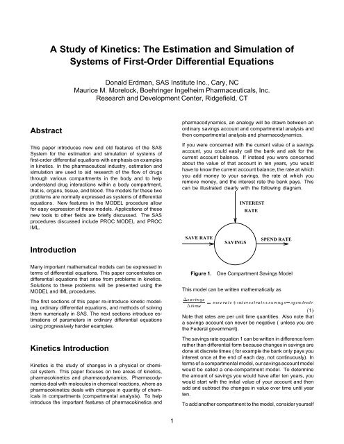
If you were concerned with the current value of a savings 

account, you could easily call the bank and ask for the 

current account balance. If instead you were concerned 

about the value of that account in ten years, you would 

have to know the current account balance, the rate at which 

you add money to your savings, the rate at which you 

remove money, and the interest rate the bank pays. This 

can be illustrated clearly with the following diagram. 

SAVE RATE 

SAVINGS 

INTEREST 

RATE 

SPEND RATE 

Figure 1. One Compartment Savings Model 

This model can be written mathematically as 

savings 

= saverate+interestrate savings,spendrate 

time 

(1) 

Note that rates are per unit time quantities. Also note that 

a savings account can never be negative ( unless you are 

the Federal government). 

The savings rate equation 1 can be written in difference form 

rather than differential form because changes in savings are 

done at discrete times ( for example the bank only pays you 

interest once at the end of each day, not continuously). In 

terms of a compartmental model, our savings account model 

would be called a one-compartment model. To determine 

the amount of savings you would have after ten years, you 

would start with the initial value of your account and then 

add and subtract the changes in value over time until year 

ten. 

To add another compartment to the model, consider yourself

as another compartment. An input to the new compartment 

would be your salary, and an output would be for taxes or 

savings. The new model could be represented as follows: 

PAY 

YOU 

MISC. 

COMPUTER 

EQUIPMENT 

TAXES 

SAVE RATE 

SAVINGS 

INTEREST 

RATE 

Figure 2. Two-Compartment Savings Model 

SPEND RATE 

In compartmental analysis, the blood stream and the stomach 

are usually considered two compartments. If a drug 

is administered orally (to the stomach), it will be absorbed 

into the blood stream at a certain rate. In order to know 

the concentration of the drug in the blood stream, you need 

to know the rate at which it leaves the stomach, the initial 

concentration in the stomach and blood, and the rate at 

which the drug is removed from the blood stream. The 

following is a diagram of this process. 

STOMACH 

ABSORB 

RATE 

BLOOD 

Figure 3. Two-Compartment Drug Model 

ELIMINATE 

RATE 

The model as is tells us only about the rate of change of 

drug concentration in two compartments. Also there are 

usually more than 6.02e23 molecules involved, so you can 

ignore the discrete nature of the number of atoms and treat 

quantity of the drug as a continuous amount. If you treat the 

quantities as continuous, a mathematical model can then 

be written in differential form rather than difference form as 

d[stomach] 

= ,rabs [stomach] (2) 

dt 

d[blood] 

= rabs [stomach] , relim [blood] (3) 

dt 

This system of differential equations can be easily solved 

analytically given values for the initial concentrations and 

values for the rate parameters. Note also that the quantity 

of the drug is conserved, and it is always positive or zero. 

The savings account problem has a major advantage over 

general compartmental models in that the value in each of 

the compartments in the savings account model is easily obtained. 

In compartmental studies, usually only one compartment 

is measured. Values in the other compartments are 

determined via the simulation of the mathematical model. 

Pharmacokinetic models, and other kinetic models, can 

always be viewed as a compartmental model. The chemical 

2 

states in a reaction can be viewed as the compartments of 

a model. 

Re-introducion to ODEs 

Ordinary differential equations, or ODE’s, are also called 

initial value problems because a time zero value for each 

first-order differential equation is needed. The following is 

an example of a first-order system of ODE’s. 

y 0 

z 0 

= ,0:1y + 2:5z 2 

(4) 

= ,z (5) 

y0 = 0 (6) 

z0 = 1 (7) 

Note that for each ODE there must be an initial value 

provided. 

As a reminder, any n-order differential equation can be 

modeled as a system of first-order differential equations. 

For example consider the following differential equation: 

y 00 

= by 0 

+ cy (8) 

y0 = 0 (9) 

y 0 

0 = 1 (10) 

which can be written as the system of differential equations: 

Model Procedure Example 

y 0 

z 0 

= z (11) 

= by 0 

+ cy (12) 

y0 = 0 (13) 

z0 = 1 (14) 

The previous differential system 11-14 can be simulated 

using the MODEL procedure as follows: 

data t; 

time=0; output; 



run; 

proc model data=t ; 

dependent y 0 z 1; 

parm b -2 c -4; 

/* Solve y’’ = b y’ + c y --------------*/ 

dert.y = z; 

dert.z = b * dert.y + c * y; 

solve y z / dynamic out=integ ; 

run; 

proc print data=integ(keep=time z y); run;

The following output was produced by the preceding statements. 

Other output produced by these statements is not 

shown. 

OBS Y Z TIME 

1 0.00000 1.00000 0 

2 0.20964 -0.26871 1 

3 -0.02476 -0.10359 2 

The differential variables are distinguished by the DERT. 

(derivative with respect to time) prefix. Once the DERT. 

variable is defined, it can be used on the right-hand side 

of another equation. The differential equations must be 

expressed in normal form; implicit differential equations are 

not allowed, and other terms on the left-hand side are not 

allowed. 

The TIME variable is the implied with respect to variable 

for all DERT. variables. The TIME variable is also the only 

variable that must be in the input data set. 

Initial values for the differential equations can be provided in 

the data set, in the declaration statement (as in the previous 

example), or in statements in the code. Using the previous 

example, you can specify the initial values as 

proc model data=t ; 

dependent y z ; 

parm b -2 c -4; 

/* Solve y’’ = b y’ + c y --------------*/ 

if ( time = 0 ) then do; 

y=0; 

z=1; 

end; 

else do; 

dert.y = z; 

dert.z = b * dert.y + c * y; 

end; 

solve y z / dynamic solveprint ; 

run; 

Simple Simulation Example 

The naturally occurring drug, Ginseng, has been a hot product 

in recent years. One of the drug’s many claims is that it 

provides the user with more energy. Ginseng is not actually 

one compound but a collection of over 1000 ingredients. 

This example models ginseng as one compound - as if all 

the ingredients act simultaneously. 

The flow of ginseng, administered orally, into and out 

of the blood stream can be modeled as follows: 

GINSENG 

IN 

CHARGE UP 

GINSENG 

IN 

DISCHARGE 

STOMACH RATE BLOOD RATE 

Figure 4. Two-Compartment Ginseng Model 

3 

This model is a simplification because you are assuming 

that all the ginseng in the stomach will be absorbed into the 

blood stream and that ginseng in the blood stream equates 

to ginseng in the effected tissues. 

This compartmental model can be written as the following 

system of differential equations: 

d [stomach] 

dt 

d [blood] 

dt 

= ,ku [stomach] (15) 

= ku [stomach] , ke [blood] (16) 

where KU is the charge up rate and KE is the discharge 

rate. Both parameters have units of 1=minutes. Given 

this model, you would like to simulate the concentration of 

ginseng in the blood stream over time. Most items sold 

commercially had to have a Manufacture Safety Data sheet 

(MSDS), which includes specifications like lethal dosages, 

vapor pressures, and so on. Using information from this 

sheet and other sources (thin air) you can get the values for 

the rate parameters KU(0.09) and KE(0.04) and an idea of 

the initial concentration in the stomach after taking two pills. 

First generate some data to drive the simulation: 

data drive; 

do time = 1 to 200 by 5; output; 

end; 

run; 

Then use the following SAS code to produce the simulation: 

proc model data=drive; 

dependent blood 0 stomach 7.2; 

parm ke 0.04 ku 0.09; 

dert.stomach = -ku * stomach; 

dert.blood = ku * stomach - ke * blood; 

solve blood stomach / out=ans dynamic; 

run; 

The following is the plot for our ginseng simulation.

Figure 5. Simulation results 

Reference lines have been added to the plot of the simulation 

results. The reference lines indicate the drug concentration 

needed to begin to have a measurable effect and 

the drug concentration that is lethal or that begins to cause 

damage in vital organs. 

Note that, according to our simplified model, ginseng was 

effective only for an hour after it was taken. These results 

are only simulated to demonstrate the software. Do not 

use these results as a basis for taking this drug. 

Simple Kinetics Estimation 

Simulation of a kinetic model requires knowledge of the 

rate parameters. In this section, estimation of the rate 

parameters in kinetic models is introduced. 

Static and Dynamic Estimation 

The default estimation method for ODE’s in the MODEL 

procedure is a static estimation. In a static estimation, 

n-1 initial value problems are solved using the first n-1 

data values as initial values. The equations are integrated 

using the ith data value as an initial value to the 

i+1 data value. See Figure 6 for a picture of how the 

residuals are computed for a static estimation of noisy data 

from a simple differential equation. For a static estimation 

the data set must contain values for the integrated 

variables. For example, if DERT.Y and DERT.Z are the 

differential variables, in order to do a static simulation 

4 

of the model, Y and Z must be in the input data set. 

Y 

ACTUAL 

INTEGRATION 

TIME 

Figure 6. Static Estimation 

To perform a dynamic estimation of the differential equation 

add the DYNAMIC option to the FIT statement. A dynamic 

estimation is obtained by solving one initial value problem 

for all the data. A graph of how the residuals are computed 

for a dynamic estimation is shown in Figure 7. 

Y 

ACTUAL 

IINTEGRATION 

TIME 

Figure 7. Dynamic Estimation 

The form of the estimation that is preferred depends mostly 

on the model and data. If the initial value is known very 

accurately, then a dynamic estimation is appropriate. If the 

model can be written analytically, then the analytical estimation 

is computationally simpler. Static estimation is less 

sensitive to errors in the initial value when an approximate 

value for the initial value is known and not modeled as 

unknown parameter. 

The form of the error in the model is also an important 

factor is choosing the method of the estimation. If the error 

term is additive and independent of previous error, then 

the dynamic model is appropriate. If, on the other hand,

the errors are cumulative, then a static estimation is more 

appropriate. 

Rate Parameter Estimation 

Consider the kinetic model for the accumulation of mercury 

(Hg) in mosquito fish ( Matis, Miller, Allen 1991, p. 177 ). 

The model for this process is the one-compartment constant 

infusion model pictured in Figure 7. 

Ku 

Fish 

Ke 

Figure 8. One-Compartment Constant Infusion Model 

The differential equation that models this process is 

d conc 

dt 

= ku , keconc (17) 

conc0 = 0 

where ku is a pseudo first order rate constant. The analytical 

solution to the model is 

The data for the model is 

data fish; 

input day conc ; 

datalines; 

0.0 0.0 

1.0000 0.1352 

2.0000 0.2168 

3.0000 0.255 

4.0000 0.3258 

6.0000 0.3313 

; 

run; 

conc =(ku=ke)(1 , exp(,ket)) (18) 

To fit this model in differential form using the MODEL 

procedure, use the following statements: 

proc model data = fish; 

parm ku ke ; 

dert.conc = ku - ke * conc; 

fit conc / time =day; 

run; 

The results from this estimation are shown in Output 1. 

Output 1. Static Estimation Results for Fish Model 

MODEL Procedure 

OLS Estimation 

Nonlinear OLS Parameter Estimates 

Approx. ’T’ Approx. 

Parameter Estimate Std Err Ratio Prob>|T| 

KU 0.173401 0.02774 6.25 0.0033 

KE 0.495189 0.10387 4.77 0.0089 

5 


18, add the dynamic option to the FIT statement. 


parm ku .3 ke .3 ; 


fit conc / time = day dynamic; 

run; 

The equation DERT.CONC is integrated from conc(0) =0. 

The results from this estimation are shown in Output 2 

Output 2. Dynamic Estimation Results for Fish Model 






KU 0.166144 0.01465 11.34 0.0003 

KE 0.459283 0.06270 7.32 0.0018 


and estimate the initial value, use the following statements: 


parm ku .3 ke .3 conc0 0; 


fit conc initial=(conc = conc0) / time =day dynamic; 

run; 

The INITIAL= option in the FIT statement is used to associate 

the initial value of a differential equation with a 

parameter. The results from this estimation are shown in 

Output 3 

Output 3. Dynamic Estimation with Initial Value for Fish 

Model 






KU 0.166092 0.02006 8.28 0.0037 

KE 0.459102 0.08163 5.62 0.0111 

CONC0 0.000074882 0.01541 0.00 0.9964 

Finally, the fish model can be estimated with the analytical 

solution by using the following statements: 


parm ku .3 ke .3; 

conc = (ku/ ke)*( 1 -exp(-ke * day)); 

fit conc ; 

run;

The results from this estimation are shown in Output 4. 

Output 4. Analytical Estimation Results for Fish Model 






KU 0.166144 0.01465 11.34 0.0003 

KE 0.459283 0.06270 7.32 0.0018 

If you Compare the results between the four estimations, the 

two dynamic estimations and the analytical estimation give 

nearly identical results (identical to the default precision). 

The two dynamic estimations are identical because the 

estimated initial value (0.00013071) is very close to the 

initial value used in the first dynamic estimation. The static 

model did not require an initial guess for the parameter 

values. Static estimation in general is more forgiving for bad 

initial values. 

IML Example 

The previous ODE example can be simulated using the IML 

subroutine ODE as follows: 

proc iml; 

start fun(t,z); 

dy = z[2]; 

dz = -2 * dy + -4 * z[1]; 

return( dy // dz ); 

finish; 

/* min and max timesteps */ 

h = {1.e-14 1 1e-5}; 

eps = 1.e-9; 

time = { 0, 1, 2 }; 

initial = { 0, 1 }; 

call ode(answer,"fun",initial,time,h) eps=eps; 

print answer; 


with the IML procedure, use the following statements: 

proc iml; 

/* define differential equation */ 

start fun(t,conc) global( ku, ke); 

dconc = ku - ke * conc; 

return( dconc ); 

finish; 

/* Function to minimize */ 

start sse( k ) global( day, conc, ku, ke ); 

/* min and max timesteps */ 

ku = k[1]; 

ke = k[2]; 

h = {1.e-14 1 1e-5}; 

6 

eps = 1.e-9; 

initial = conc[1]; 

call ode(answer,"fun",initial,day,h) eps=eps; 

/* get sse */ 

r = answer‘ - conc[2:6,]; 

sse = r‘ * r; 

return(sse); 

finish; 

use fish; 

read all var{day conc}; 

ku = 0.3; 

ke = 0.3; 

k = ku // ke; 

optn = {0 3}; 

call nlpqn(rc,est,"sse",k, optn); 

print est; 

run; 

IML versus MODEL 

The IML and MODEL procedures use the same underlying 

routines to perform the integration. The major difference 

between the two procedures is that the MODEL procedure 

automatically computes the analytical derivatives of the 

ODE’s with respect to the parameters. The derivatives of 

the ODE’s with respect to the parameters turn out to be 

themselves ODE’s which must be integrated along with the 

original system. Because of limitations in machine precision, 

numerically integrated values can be, at best, accurate to 

10 decimal places. 

Besides the obvious syntax differences between the IML 

and MODEL procedures, there are three important advantages 

to using the MODEL procedure. The first advantage 

is that the MODEL procedure computes the derivatives 

needed for solving and estimating the system analytically 

and automatically. The IML procedure either uses numerical 

differencing or user supplied analytical derivatives. If 

numerical differencing is used for the derivatives needed 

for estimation, the combination of the numerical integration 

truncation errors and the differencing truncation error restricts 

the stiffness of the problems that can be estimated. 

Stiffness here refers to the differences in the magnitudes of 

the estimated rate parameters. 

The second advantage that the MODEL procedure has 

for ODE’s is that it scales the numerical integration. The 

scaling is done dynamically and ensures that the integration 

remains well behaved and defined. The third advantage 

is that the structure of the Jacobian (used in solving the 

system of ODE’s) is exploited to significantly speed up the 

integration process in the estimation phase. 

Differential/Algebraic Equations 

In kinetics models it is sometimes easier to use conservation 

equations to express relations between concentrations. 

Conservation equations also have the advantage of not

having rate constants that must be known or estimated. 

Equations in a system that express algebraic relations (as 

opposed to differential ) and are need to do the integration 

are call auxiliary equations. Adding auxiliary equations to 

a system of ordinary differential equations turns the system 

into a differential/algebraic system (DAS). 

Consider the following example: 

The Michaelis-Menten Equations describe the kinetics of an 

enzyme-catalyzed reaction. E is the enzyme, and S is called 

the substrate. The enzyme first reacts with the substrate to 

form the enzyme-substrate complex ES, which then breaks 

down in a second step to form enzyme and products P. 

The reaction rates are described by the following system of 

differential equations: 

d[ES] 

dt 

= k1[E][S] , k2[ES] , k3[ES] (19) 

d[S] 

dt 

= ,k1[E][S]+k2[ES] (20) 

[E] = [E]tot , [ES] (21) 

The first equation describes the rate of formation of ES from 

E + S. ( The rate of formation of ES from E + P is very small 

and can be ignored.) The enzyme is in either the complexed 

or uncomplexed form. So if the total ([E]tot) concentration of 

enzyme and the amount bound to the substrate are known, 

the concentration of the unbound enzyme can be obtained 

by conservation. 

In this example the conservation equation is an auxiliary 

equation and will be coupled with the differential equations 

for integration. 

More Complex Example 

The following is a simplified reaction scheme for the competitive 

inhibitors with recombinant human renin (Morelock 

and others 1995) 

k2r 

E + D 

+ 

I 

EI 

k2f 

k1f 

k1r 

ED 

Figure 9. Competitive Inhibition of Recombinant Human 

Renin 

where E = enzyme, D = probe, and I = inhibitor. The 

differential equations describing this reaction scheme are 

7 

dD 

dt 

dED 

dt 

dE 

dt 

dEI 

dt 

dI 

dt 

= k1r ED , k1f E D (22) 

= k1f E D , k1r ED 

= k1r ED , k1f E D + k2r EI , k2f E I 

= k2f E I , k2r EI 

= k2r EI , k2f E I 

For this system, the initial values for the concentrations are 

derived from equilibrium considerations (as a function of 

parameters) or are provided as known values. 

The experiment used to collect the data was carried out 

in two phases: pre-incubation of the probe with enzyme 

(type=’dis’) and pre-incubation of the inhibitor with enzyme 

(type=’ass). Both reaction phases were initiated by addition 

of the complementary ligand. The data also contain 

repeated measurements. The data contain values for fluorescence 

F, which is a function of concentration. Since there 

are no direct data for the concentrations, all the differential 

equations are simulated dynamically. 

The SAS statements used to fit this model are 

PROC MODEL DATA=renin ; 

parameters qf = 2.1e8 

qb = 4.0e9 

k2f = 1.8e5 

k2r = 2.1e-3 

L = 0; 

/* Known parameter values -----------------*/ 

k1f = 6.85e6 ; 

k1r = 3.43e-4 ; 

/* Initial values for concentrations */ 

control dt 5.0e-7 

et 5.0e-8 

it 8.05e-6; 

/* Association initial values --------------*/ 

if type = ’ass’ and time=0 then do ; 

ed = 0 ; 

/* solve quadratic equation ----------*/ 

a = 1 ; 

b = -( it + et + ( k2r / k2f )) ; 

c = it*et ; 

ei =(-b-((( b**2 )-(4 * a * c ))**.5))/( 2*a ); 

d = dt - ed ; 

i = it - ei ; 

e = et - ed - ei ; 

end ; 

/* Disassociation initial values ----------*/ 

if type = ’dis’ and time=0 then do ; 

ei = 0 ; 

a = 1 ; 

b = -( dt + et + ( k1r / k1f)) ; 

c = dt * et ; 

ed =(-b-((( b**2 )-(4 * a * c ))**.5))/( 2*a ); 

d = dt - ed ; 

i = it - ei ;

un; 

e = et - ed - ei ; 

end ; 

if time ne 0 then do; 

dert.d = k1r * ed - k1f * e * d; 

dert.ed = k1f * e * d - k1r * ed; 

dert.e = k1r * ed - k1f * e * d 

+ k2r * ei - k2f * e * i; 

dert.ei = k2f * e * i - k2r * ei; 

dert.i = k2r * ei - k2f * e * i; 

end; 

/* L - offset between curves */ 

if type = ’dis’ then 

F = ( qf * (d - ed)) + ( qb * ed ) - L; 

else 

F = ( qf * (d - ed)) + ( qb * ed ) ; 

Fit F / method=marquardt dynamic; 

The results of the estimation are shown in Output 5. 

Output 5. Kinetics Estimation 



Nonlinear OLS Summary of Residual Errors 

DF DF 

Equation Model Error SSE MSE Root MSE 

F 5 797 2525 3.16814 1.77993 






QF 204127823 681444.7 299.55 0.0001 

QB 4226271902 9133182.6 462.74 0.0001 

K2F 6451854.40 867169.3 7.44 0.0001 

K2R 0.00780873 0.0010350 7.54 0.0001 

L -5.770088 0.41379 -13.94 0.0001 

In the paper by Morelock and others (1995), this differential 

system was estimated using an analytical solution to the 

system. The estimated parameters for the analytical equations 

and the ODE’s were identical, though it took many 

more man hours to come up with the correct analytical 

equations. 

Computational Complexities 

In the preceding example, the estimation of the parameters 

requires the repeated simulation of a system of 42 

differential equations ( 5 base differential equations and 36 

8 

differential equations to compute the partials with respect 

to the parameters). In addition to being evaluated at each 

data point, the model is evaluated at multiple points between 

each data point to ensure an accurate integration. 

Estimations can take a couple of seconds to a couple of 

hours. 

It is important to note that most kinetics estimations will have 

multiple solutions if data for all compartments or concentrations 

are not known. So it is crucial that other information 

about the problem be known in order to determine the 

proper answer. For linear systems, it is sufficient to know 

the relative magnitudes of the rate parameters in order to 

determine a unique parameter set. A BOUNDS statement 

can be used to enforce that restriction. 

Summary 

This paper provided an overview of the SAS procedures 

MODEL and IML that can be used to solve and estimate 

nonlinear systems of ordinary differential equations. The examples 

emphasized ODE’s arising from problems in pharmacokinetics 

even though the capabilities are not limited to 

problems in those fields. 

References 

Aiken, R.C., ed. (1985), Stiff Computation, New York: 

Oxford University Press. 

Byrne, G.D. and Hindmarsh, A.C. (March 1975), “A Polyalgorithm 

for the Numerical Solution of ODE’s,” in ACM 

TOMS, 1(1), 71-96. 

Matis, J.H., Miller, T.H., and Allen, D.M. (1991), Metal 

Ecotoxicology Concepts and Applications, eds. M.C 

Newman and Alan W. McIntosh , Michigan: Lewis 

Publishers Inc. 

Morelock, M.M. Pargellis, C. A., Graham, E.T., Lamarre, D., 

and Jung, G. (1995), “Time-Resolved Ligand Exchange 

Reactions: Kinetic Models for Competitive Inhibitors 

with Recombinant Human Renin ,” Journal of Medical 

Chemistry, 38, 1751-1761.

A Study of Kinetics: The Estimation and Simulation of Systems of - SAS

Create successful ePaper yourself

Delete template?

Save as template?