329-2012: Dynamically Evolving Systems: Cluster Analysis ... - SAS

SAS Global Forum 2012 

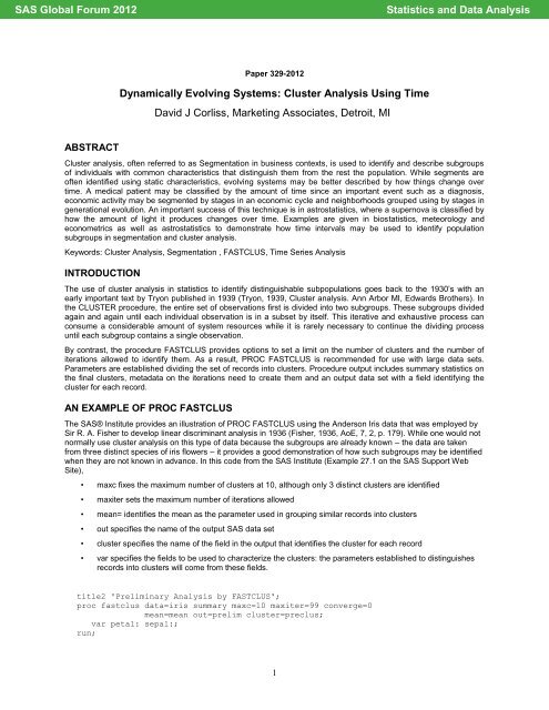
ABSTRACT 

Paper 329-2012 

Dynamically Evolving Systems: Cluster Analysis Using Time 

David J Corliss, Marketing Associates, Detroit, MI 

Cluster analysis, often referred to as Segmentation in business contexts, is used to identify and describe subgroups 

of individuals with common characteristics that distinguish them from the rest the population. While segments are 

often identified using static characteristics, evolving systems may be better described by how things change over 

time. A medical patient may be classified by the amount of time since an important event such as a diagnosis, 

economic activity may be segmented by stages in an economic cycle and neighborhoods grouped using by stages in 

generational evolution. An important success of this technique is in astrostatistics, where a supernova is classified by 

how the amount of light it produces changes over time. Examples are given in biostatistics, meteorology and 

econometrics as well as astrostatistics to demonstrate how time intervals may be used to identify population 

subgroups in segmentation and cluster analysis. 

Keywords: Cluster Analysis, Segmentation , FASTCLUS, Time Series Analysis 

INTRODUCTION 

The use of cluster analysis in statistics to identify distinguishable subpopulations goes back to the 1930’s with an 

early important text by Tryon published in 1939 (Tryon, 1939, Cluster analysis. Ann Arbor MI, Edwards Brothers). In 

the CLUSTER procedure, the entire set of observations first is divided into two subgroups. These subgroups divided 

again and again until each individual observation is in a subset by itself. This iterative and exhaustive process can 

consume a considerable amount of system resources while it is rarely necessary to continue the dividing process 

until each subgroup contains a single observation. 

By contrast, the procedure FASTCLUS provides options to set a limit on the number of clusters and the number of 

iterations allowed to identify them. As a result, PROC FASTCLUS is recommended for use with large data sets. 

Parameters are established dividing the set of records into clusters. Procedure output includes summary statistics on 

the final clusters, metadata on the iterations need to create them and an output data set with a field identifying the 

cluster for each record. 

AN EXAMPLE OF PROC FASTCLUS 

The SAS® Institute provides an illustration of PROC FASTCLUS using the Anderson Iris data that was employed by 

Sir R. A. Fisher to develop linear discriminant analysis in 1936 (Fisher, 1936, AoE, 7, 2, p. 179). While one would not 

normally use cluster analysis on this type of data because the subgroups are already known – the data are taken 

from three distinct species of iris flowers – it provides a good demonstration of how such subgroups may be identified 

when they are not known in advance. In this code from the SAS Institute (Example 27.1 on the SAS Support Web 

Site), 

• maxc fixes the maximum number of clusters at 10, although only 3 distinct clusters are identified 

• maxiter sets the maximum number of iterations allowed 

• mean= identifies the mean as the parameter used in grouping similar records into clusters 

• out specifies the name of the output SAS data set 

• cluster specifies the name of the field in the output that identifies the cluster for each record 

• var specifies the fields to be used to characterize the clusters: the parameters established to distinguishes 

records into clusters will come from these fields. 

title2 'Preliminary Analysis by FASTCLUS'; 

proc fastclus data=iris summary maxc=10 maxiter=99 converge=0 

mean=mean out=prelim cluster=preclus; 

var petal: sepal:; 

run; 

1 

Statistics and Data Analysis


As the output from the SAS Institute example shows, the data are divided into three clusters; thee groups closely 

match the distribution of the three botanical species that make up the Anderson data. 

Figure 1: Cluster Analysis of Anderson Iris Data 

CLUSTER ANALYSIS APPLIED TO TIME SERIES DATA 

A dynamically evolving system is one that changes over time, often going through distinct steps or stages as it 

changes. One example of a dynamically evolving system is the seasonal variation in weather. In this example, the 

start and end dates of four annual weather seasons in the state of Michigan are identified by applying PROC 

FASTCLUS using precipitation data from the National Oceanic and Atmospheric Administration. In these data, the 

year and month are contained in a single field and must be parsed before the executing the PROC FASTCLUS. The 

use of NOAA weather data to demonstrate cluster analysis of time series data follows a homework problem 

presented by Dr. Robert Fovell in the Department of Atmospheric and Oceanic Sciences at UCLA. 

**** NOAA Precipitation Data ****; 

data work.noaa; 

infile "/home/sas/NESUG/noaa_mi_1950_2009_tab.txt" 

dsd dlm='09'x lrecl=1500 truncover firstobs=2; 

input 

state_code :3.0 

division :3.0 

year_month :$6. 

pcp :6.2 

; 

length year 8.0 month 8.0; 

year = left(year_month,1,4); 

month = right(year_month,5,2); 

run; 

In using PROC FASTCLUS on time series data, the time variable appears first in the VAR statement. This leads SAS 

create the first split of the data by starting at the opposite ends of the time series and working towards the middle. If 

there is if sufficient discrimination into distinct groups with different characteristics, the time series will be divided in 

half with the break between the group clusters at the median date. Therefore, an initial run is made with only two 

clusters (maxc=2) to test whether the data is being properly divided into groups that are genuinely different instead of 

being arbitrarily divided in half at the middle. 

2 



proc fastclus data=work.noaa maxc=2 maxiter=10 out=work.cluster1; 

var month pcp; 

run; 

Running the PROC FASTCLUS with maxc=4 gives the desired four seasons: 

proc fastclus data=work.noaa maxc=4 maxiter=10 out=work.cluster3; 

var month pcp; 

run; 

Time series data can be plotted to display the successive steps in the time series identified by the different clusters. 

The use of small, square markers for individual records facilitates display of the time series as a line of color changing 

over time. 

goptions device=png; 

symbol1 font=marker value=u height=0.6 c=blue; 

symbol2 font=marker value=u height=0.6 c=red; 

symbol3 font=marker value=u height=0.6 c=yellow; 

symbol4 font=marker value=u height=0.6 c=green; 

legend1 frame cframe=ligr label=none cborder=black position=center 

value=(justify=center); 

axis1 label=(angle=90 rotate=0) minor=none; 

axis2 minor=none; 

proc gplot data=work.cluster3; 

plot year * month = cluster /frame cframe=ligr 

legend=legend1 vaxis=axis1 haxis=axis2; 

run; 

Figure 2: Seasonal Variation in Precipitation in the State of Michigan, 1950-2009 (NOAA Data) 

3 



In this plot, the annual seasonal changes in precipitation by month are reflected in the clusters identified in this 

analysis. Changes in the beginning, end and / or duration of seasons over a period of years may reflect climate 

change. 

USE OF THE STANDARD PROCEDURE 

In the next example, from econometrics, seasonal changes in gas prices are investigated. Archived weekly national 

average prices for gasoline from the United States Department of Energy / Energy Information Administration are 

used to identify time series clusters reflecting what we all pay at the pump. Unlike the amount of rain in a year, the 

price of a commodity will steadily increase over time. Fields with larger variances are given more weight in 

determining clusters. Also, if average value of a field steadily increases or decreases over time, the weight that field is 

given will also change. Use of the SAS procedure STANDARD before executing the cluster analysis corrects for this 

by normalizing fields to the total amount of variation for each field in the data set. 

The time series of gasoline supply and price, like that of many other commodities, is autocorrelated, with values in the 

short-term future as more strongly correlated to values in the recent past than to those in the more distant past. In this 

case, the time rate of change of some property may better characterize the behavior than values observed at one 

moment in time. It is therefore can be important in time series analysis to include the rate of change of critical fields in 

addition to their values. In this example, a RETAIN statement is used to capture and preserve the values for price and 

supply for from the previous week and the weekly percent change in these values is calculated. The calculation of 

ordinal week from the date of a record is also included. 

**** doe gas price data ****; 

data work.doe; 

infile "/home/sas/doe_prices.txt" dsd dlm='09'x lrecl=80 truncover firstobs=2; 

input date :mmddyy10. price :8.2; 

year = year(date); 

week = round((((date + 3) - mdy(1,1,year)) / 7),1); 

if week ge 1 and week le 52; 

run; 

**** normalize gas prices to annual mean ****; 

proc sort data=work.doe; 

by year week; 

run; 

proc univariate data=work.doe noprint; 

by year; 

var price; 

output mean=annual_mean_price out=work.annual; 

run; 


merge work.doe work.annual; 

by year; 

annualized_price_index = price / annual_mean_price; 

run; 

**** interval percent change ****; 

proc sort data=work.doe; 

by year week; 

run; 


set work.doe; 

by year week; 

retain pw_price_index; output; 

if first.week then pw_price_index = annualized_price_index; 

run; 

4 




set work.doe; 

by year week; 

weekly_pct_change = (annualized_price_index - pw_price_index) * 100; 

run; 

PROC STANDARD is used to normalized to the values of fields to be used later in PROC FASTCLUS: 

proc standard data=work.doe mean=0 std=1 out=work.doe_stan; 

var week annualized_price_index weekly_pct_change supply supply_pct_change; 

run; 

proc fastclus data=work.doe_stan maxc=6 maxiter=20 out=work.cluster1; 


run; 

Figure 3: Seasonal Cluster Analysis of US Gasoline Prices, 1991-2010 

In this set of clusters, both seasonal variation over a single year as well as historical changes of the course of several 

years are indicated. Cluster #3 dominates the early part of the year for all years in this study. However, the 

dominance of #1 late in the year during the early- and mid-1990’s is later replaced by #2, followed by #5 in many 

years. This indicates that the annual pattern of seasonal variations may have gradually changed over the past 20 

years. 

By averaging together the normalized fields for each week, a single line of time series clusters is used to identify 

benchmarks for the timing and amount of change seen over the course of an average year: 

5 



proc sort data=work.doe2; 

by week; 

run; 

proc means data=work.doe2 noprint; 

by week; 

var annualized_price_index weekly_pct_change supply supply_pct_change; 

output out=work.doe_week; 

run; 

data work.doe_week; 

set work.doe_week; 

by week; 

if _stat_ = 'mean'; 

keep week annualized_price_index weekly_pct_change supply supply_pct_change; 

run; 

proc standard data=work.doe_week mean=0 std=1 out=work.doe_stan; 


run; 

proc fastclus data=work.doe_stan maxc=6 maxiter=20 out=work.cluster1; 


run; 

Figure 4: Averaged Seasonal Cluster Analysis of US Gasoline Prices, 1991-2010 

In this set of clusters, we see a post-holiday lull in the first week of the year (cluster #1), a winter season with low 

prices and abundant supply (#5), a run-up of prices and supply shortages from mid-March through the end of May 

when refineries are changing over from winter formulations to summer (#2), a summer driving season with significant 

supply but higher demand and occasional spikes (#3 and #6) and a gradual decline in prices from mid-September - 

December (#4). 

ANALYSIS OF ONE-TIME EVENTS AND PROCESSES OF VARIABLE DURATION 

Of course, not all events repeat on an annual cycle. The period of repetition for those that cycle over a different time 

scale can be found by spectral analysis (see the SPECTRA procedure). With the period of repetition known, the time 

series cluster analysis can proceed as described above. 

However, many occurrences are not cyclical over any period. A given stock-split, hospital visit or supernova will only 

happen once but all these may have a characteristic series steps that following in the same order as they unfold. 

Supernovae provide an excellent instance of one-time events that can be classified into different types by how a 

critical property – in this case, the amount of light they produce – changes over time. Time series clusters, each 

representing a separate evolutionary stage of development , can be determined by matching their time series to other 

similar events seen in the past. 

While some one-time events last for a standard length of time, the most general case is given by events that follow an 

exact sequence but vary in overall duration. In astrophysics, the violent stellar eruptions known as High Velocity 

Absorption (HVA) events seen in certain hot stars appear to follow a definite sequence but vary in duration by an 

order of magnitude or more. This present work in time series cluster analysis originally was undertaken to identify the 

evolutionary stages of these one-time events of variable duration. 

6 



In the analysis of events with variable duration, the time values are re-normalized using the difference between two 

benchmark points in time. Often, as in the case of HVAs, the beginning and the end of the event provide the overall 

duration. The time points are then re-cast as a percent of the time from beginning to end. In this analysis of HVAs, the 

initial and final dates are extracted and then merged with each record. The percent of the total time elapsed from the 

beginning is calculated and then used as the time variable in the cluster analysis. 

**** astrophysics data - time series of high velocity absorption events ****; 

data work.first_date; 

set work.hva; 

by event_id jd_minus_24e5; 

if first.event_id; 

first_date = jd_minus_24e5; 

keep event_id first_date; 

run; 

(and similarly for the last date of each event, which are merged with the first 

date) 

data work.hva; 

merge work.hva work.first_last; 

by event_id; 

percent_duration = (day_of_event / duration) * 100; 

run; 

The time series cluster analysis then proceeds as before, with PROC STANDARD to normalize the fields followed 

PROC FASTCLUS. HVAs appear to go through up to four distinct stages, so this was set as the number of clusters in 

the procedure. In Time Series Analysis, whether to use absolute or relative measures is often an important 

consideration. Absolute measures give the value of some property at each point in time, while relative measures give 

the rate at which the value of the property is changing. It is generally advisable to investigate both time absolute and 

relative measures to determine the combination of observables that best match the data. 

proc standard data=work.hva mean=0 std=1 out=work.hva_stan; 

var percent_duration eq_width_absorp delta_rate; 

run; 

proc fastclus data=work.hva_stan maxc=4 maxiter=10 out=work.cluster1; 

var percent_duration eq_width_absorp delta_rate; 

run; 

In this case of HVAs in late B- and early A-type stars, the best separation of clusters was given when both the 

observed values and their rates of changes were included in the analysis: 

Figure 5: Comparison of Magnitude vs. Time Rate of Change Variables in Cluster Analysis 

7 



The first stage in these events, represented by Cluster #1, is a characterized by an rapid increase in the quantity and 

velocity of material ejected from the star while the absolute amounts remain fairly small (#1), followed by a rise to a 

sharp peak (#2) and then a rapid decrease of 60%-70% (#3). Following an interval with little change, a final drop back 

down to zero intensity is observed (#4). Once the clusters have been identified, the data may be plotted with colors 

indicating the clusters: 

Figure 6: Evolutionary Stages in High Velocity Absorption Events in the A0 Supergiant Star HR 1040 

CONCLUSION 

The SAS procedures developed for cluster analysis can be applied to events that change over time to identify distinct, 

successive stages in dynamically evolving systems. Both cyclical and non-repeating events may be analyzed. 

Normalization of fields through the use of PROC STANDARD may be necessary prior to cluster analysis to obtain the 

best results. 

REFERENCES 

Fisher, R.A., 1936, Annals of Eugenics, 7, 2, 179 

Tryon, R. C., 1939, Cluster analysis. Ann Arbor: Edwards Brothers 

CONTACT INFORMATION 

Your comments and questions are valued and encouraged. Contact the author at: 

David J Corliss 

Marketing Associates LLC 

1 Kennedy Square, Suite 500 

Detroit, MI 48224 

313.202.6323 

8 



dcorliss@marketingassociates.com 

www.marketingassociates.com 

Department of Physics and Astronomy, Mailstop 111 

The University of Toledo 

2801 West Bancroft Street 

Toledo, OH 43606 

419.530.2241 

dcorliss@marketingassociates.com 

www.marketingassociates.com 

davidjcorliss@rockets.utoledo.edu 

http://astro1.panet.utoledo.edu/~dcorliss/ 

SAS and all other SAS Institute Inc. product or service names are registered trademarks or trademarks of SAS 

Institute Inc. in the USA and other countries. ® indicates USA registration. 

Other brand and product names are trademarks of their respective companies. 

9

329-2012: Dynamically Evolving Systems: Cluster Analysis ... - SAS

You also want an ePaper? Increase the reach of your titles

Delete template?

Save as template?