329-2012: Dynamically Evolving Systems: Cluster Analysis ... - SAS

SAS Global Forum 2012
In this plot, the annual seasonal changes in precipitation by month are reflected in the clusters identified in this
analysis. Changes in the beginning, end and / or duration of seasons over a period of years may reflect climate
change.
USE OF THE STANDARD PROCEDURE
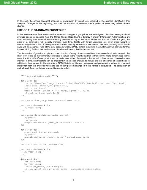
In the next example, from econometrics, seasonal changes in gas prices are investigated. Archived weekly national
average prices for gasoline from the United States Department of Energy / Energy Information Administration are
used to identify time series clusters reflecting what we all pay at the pump. Unlike the amount of rain in a year, the
price of a commodity will steadily increase over time. Fields with larger variances are given more weight in
determining clusters. Also, if average value of a field steadily increases or decreases over time, the weight that field is
given will also change. Use of the SAS procedure STANDARD before executing the cluster analysis corrects for this
by normalizing fields to the total amount of variation for each field in the data set.
The time series of gasoline supply and price, like that of many other commodities, is autocorrelated, with values in the
short-term future as more strongly correlated to values in the recent past than to those in the more distant past. In this
case, the time rate of change of some property may better characterize the behavior than values observed at one
moment in time. It is therefore can be important in time series analysis to include the rate of change of critical fields in
addition to their values. In this example, a RETAIN statement is used to capture and preserve the values for price and
supply for from the previous week and the weekly percent change in these values is calculated. The calculation of
ordinal week from the date of a record is also included.
**** doe gas price data ****;
data work.doe;
infile "/home/sas/doe_prices.txt" dsd dlm='09'x lrecl=80 truncover firstobs=2;
input date :mmddyy10. price :8.2;
year = year(date);
week = round((((date + 3) - mdy(1,1,year)) / 7),1);
if week ge 1 and week le 52;
run;
**** normalize gas prices to annual mean ****;
proc sort data=work.doe;
by year week;
run;
proc univariate data=work.doe noprint;
by year;
var price;
output mean=annual_mean_price out=work.annual;
run;
data work.doe;
merge work.doe work.annual;
by year;
annualized_price_index = price / annual_mean_price;
run;
**** interval percent change ****;
proc sort data=work.doe;
by year week;
run;
data work.doe;
set work.doe;
by year week;
retain pw_price_index; output;
if first.week then pw_price_index = annualized_price_index;
run;
4
Statistics and Data Analysis