423-2013: Computing Direct and Indirect Standardized Rates ... - SAS
423-2013: Computing Direct and Indirect Standardized Rates ... - SAS
423-2013: Computing Direct and Indirect Standardized Rates ... - SAS

You also want an ePaper? Increase the reach of your titles
YUMPU automatically turns print PDFs into web optimized ePapers that Google loves.
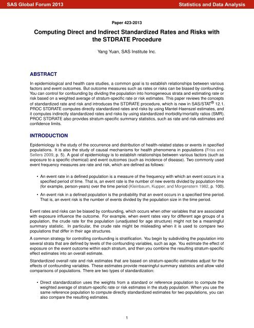
<strong>SAS</strong> Global Forum <strong>2013</strong><br />
Paper <strong>423</strong>-<strong>2013</strong><br />
<strong>Computing</strong> <strong>Direct</strong> <strong>and</strong> <strong>Indirect</strong> St<strong>and</strong>ardized <strong>Rates</strong> <strong>and</strong> Risks with<br />
the STDRATE Procedure<br />
ABSTRACT<br />
Yang Yuan, <strong>SAS</strong> Institute Inc.<br />
In epidemiological <strong>and</strong> health care studies, a common goal is to establish relationships between various<br />
factors <strong>and</strong> event outcomes. But outcome measures such as rates or risks can be biased by confounding.<br />
You can control for confounding by dividing the population into homogeneous strata <strong>and</strong> estimating rate or<br />
risk based on a weighted average of stratum-specific rate or risk estimates. This paper reviews the concepts<br />
of st<strong>and</strong>ardized rate <strong>and</strong> risk <strong>and</strong> introduces the STDRATE procedure, which is new in <strong>SAS</strong>/STAT ® 12.1.<br />
PROC STDRATE computes directly st<strong>and</strong>ardized rates <strong>and</strong> risks by using Mantel-Haenszel estimates, <strong>and</strong><br />
it computes indirectly st<strong>and</strong>ardized rates <strong>and</strong> risks by using st<strong>and</strong>ardized morbidity/mortality ratios (SMR).<br />
PROC STDRATE also provides stratum-specific summary statistics, such as rate <strong>and</strong> risk estimates <strong>and</strong><br />
confidence limits.<br />
INTRODUCTION<br />
Epidemiology is the study of the occurrence <strong>and</strong> distribution of health-related states or events in specified<br />
populations. It is also the study of causal mechanisms for health phenomena in populations (Friss <strong>and</strong><br />
Sellers 2009, p. 5). A goal of epidemiology is to establish relationships between various factors (such as<br />
exposure to a specific chemical) <strong>and</strong> event outcomes (such as incidence of disease). Two commonly used<br />
event frequency measures are rate <strong>and</strong> risk, which are defined as follows:<br />
• An event rate in a defined population is a measure of the frequency with which an event occurs in a<br />
specified period of time. That is, an event rate is the number of new events divided by population-time<br />
(for example, person-years) over the time period (Kleinbaum, Kupper, <strong>and</strong> Morgenstern 1982, p. 100).<br />
• An event risk in a defined population is the probability that an event occurs in a specified time period.<br />
That is, an event risk is the number of events divided by the population size in the time period.<br />
Event rates <strong>and</strong> risks can be biased by confounding, which occurs when other variables that are associated<br />
with exposure influence the outcome. For example, when event rates vary for different age groups of a<br />
population, the crude rate for the population (unadjusted for age structure) might not be a meaningful<br />
summary statistic. In particular, the crude rate might be misleading when it is used to compare two<br />
populations that differ in their age structures.<br />
A common strategy for controlling confounding is stratification. You begin by subdividing the population into<br />
several strata that are defined by levels of the confounding variables, such as age. You estimate the effect of<br />
exposure on the event outcome within each stratum, <strong>and</strong> then you combine the resulting stratum-specific<br />
effect estimates into an overall estimate.<br />
St<strong>and</strong>ardized overall rate <strong>and</strong> risk estimates that are based on stratum-specific estimates adjust for the<br />
effects of confounding variables. These estimates provide meaningful summary statistics <strong>and</strong> allow valid<br />
comparisons of populations. There are two types of st<strong>and</strong>ardization:<br />
• <strong>Direct</strong> st<strong>and</strong>ardization uses the weights from a st<strong>and</strong>ard or reference population to compute the<br />
weighted average of stratum-specific rate or risk estimates in the study population. When you use the<br />
same reference population to compute directly st<strong>and</strong>ardized estimates for two populations, you can<br />
also compare the resulting estimates.<br />
1<br />
Statistics <strong>and</strong> Data Analysis
<strong>SAS</strong> Global Forum <strong>2013</strong><br />
• <strong>Indirect</strong> st<strong>and</strong>ardization uses the stratum-specific rate or risk estimates in the reference population to<br />
compute the expected number of events in the study population. The ratio of the observed number<br />
of events to the computed expected number of events in the study population is the st<strong>and</strong>ardized<br />
morbidity ratio (SMR). SMR is also the st<strong>and</strong>ardized mortality ratio if the event is death; you can use it<br />
to compare rates or risks between the study <strong>and</strong> reference populations.<br />
The STDRATE (pronounced “st<strong>and</strong>ard rate”) procedure provides both directly st<strong>and</strong>ardized <strong>and</strong> indirectly<br />
st<strong>and</strong>ardized rate <strong>and</strong> risk estimates. In addition, if an effect (such as the rate difference between two<br />
populations) is homogeneous across strata, PROC STDRATE also provides the Mantel-Haenszel method<br />
(Greenl<strong>and</strong> <strong>and</strong> Rothman 2008, p. 271) to compute a pooled estimate of the effect that is based on these<br />
stratum-specific effect estimates.<br />
Note: The term st<strong>and</strong>ardization has different meanings in other statistical applications. For example, the<br />
STANDARD procedure st<strong>and</strong>ardizes numeric variables in a <strong>SAS</strong> data set to a given mean <strong>and</strong> st<strong>and</strong>ard<br />
deviation.<br />
The following three sections describe the main features of PROC STDRATE: direct st<strong>and</strong>ardization, Mantel-<br />
Haenszel estimation, <strong>and</strong> indirect st<strong>and</strong>ardization <strong>and</strong> SMR. Each section includes an example. These<br />
sections are followed by a summary section that summarizes the main features of PROC STDRATE.<br />
DIRECT STANDARDIZATION<br />
<strong>Direct</strong> st<strong>and</strong>ardization uses the weights from a st<strong>and</strong>ard or reference population to compute the weighted<br />
average of stratum-specific estimates in the study population. The directly st<strong>and</strong>ardized rate is computed as<br />
P<br />
O j<br />
ds D<br />
Trj O sj<br />
Tr<br />
where O sj is the rate in the jth stratum of the study population, Trj is the population-time in the jth stratum of<br />
the reference population, <strong>and</strong> Tr D P<br />
k Trk is the total population-time in the reference population.<br />
The st<strong>and</strong>ardized risk can also be computed similarly.<br />
The direct st<strong>and</strong>ardization is applicable when the study population is large enough to provide stable stratumspecific<br />
estimates. The directly st<strong>and</strong>ardized estimate is the overall crude estimate in the study population if<br />
it has the same strata distribution as the reference population.<br />
When you use the same reference population to derive st<strong>and</strong>ardized estimates for different populations, you<br />
can also use the estimated difference <strong>and</strong> estimated ratio statistics to compare the resulting estimates.<br />
EXAMPLE: COMPARING DIRECTLY STANDARDIZED RATES<br />
This example computes directly st<strong>and</strong>ardized mortality rates for populations in the states of Alaska <strong>and</strong><br />
Florida, <strong>and</strong> then compares these two st<strong>and</strong>ardized rates with a rate ratio statistic.<br />
The following Alaska data set contains the stratum-specific mortality information in a given period of time for<br />
the state of Alaska (Alaska Bureau of Vital Statistics 2000a, b):<br />
data Alaska;<br />
State='Alaska';<br />
input Sex $ Age $ Death PYear comma9.;<br />
datalines;<br />
Male 00-14 37 81,205<br />
Male 15-34 68 93,662<br />
Male 35-54 206 108,615<br />
Male 55-74 369 35,139<br />
Male 75+ 556 5,491<br />
Female 00-14 78 77,203<br />
Female 15-34 181 85,412<br />
Female 35-54 395 100,386<br />
Female 55-74 555 32,118<br />
Female 75+ 479 7,701<br />
;<br />
2<br />
Statistics <strong>and</strong> Data Analysis
<strong>SAS</strong> Global Forum <strong>2013</strong><br />
The variables Sex <strong>and</strong> Age are the grouping variables that form the strata in the st<strong>and</strong>ardization, <strong>and</strong> the<br />
variables Death <strong>and</strong> PYear indicate the number of events <strong>and</strong> person-years, respectively. The COMMA9.<br />
format is specified in the DATA step to input numerical values that contain commas in PYear.<br />
The following Florida data set contains the corresponding stratum-specific mortality information for the state<br />
of Florida (Florida Department of Health 2000, 2012):<br />
data Florida;<br />
State='Florida';<br />
input Sex $ Age $ Death comma8. PYear comma11.;<br />
datalines;<br />
Male 00-14 1,189 1,505,889<br />
Male 15-34 2,962 1,972,157<br />
Male 35-54 10,279 2,197,912<br />
Male 55-74 26,354 1,383,533<br />
Male 75+ 42,443 554,632<br />
Female 00-14 906 1,445,831<br />
Female 15-34 1,234 1,870,430<br />
Female 35-54 5,630 2,246,737<br />
Female 55-74 18,309 1,612,270<br />
Female 75+ 53,489 868,838<br />
;<br />
The crude rate for Alaska (2924/626932 = 0.004664) is less than the crude rate for Florida (76455/15577105<br />
= 0.004908). However, because the age distributions in the two states differ widely, these crude rates might<br />
not provide a valid comparison.<br />
To compare st<strong>and</strong>ardized rates for the two populations, you can combine the two data sets to form a single<br />
data set to be used in the DATA= option. The following TwoStates data set contains the data sets Alaska <strong>and</strong><br />
Florida, where the variable State identifies the two states:<br />
data TwoStates;<br />
length State $ 7.;<br />
set Alaska Florida;<br />
run;<br />
The following US data set contains the stratum-specific person-years information for the United States (U.S.<br />
Bureau of the Census 2011):<br />
data US;<br />
input Sex $ Age $ PYear comma12.;<br />
datalines;<br />
Male 00-14 30,854,207<br />
Male 15-34 40,199,647<br />
Male 35-54 40,945,028<br />
Male 55-74 19,948,630<br />
Male 75+ 6,106,351<br />
Female 00-14 29,399,168<br />
Female 15-34 38,876,268<br />
Female 35-54 41,881,451<br />
Female 55-74 22,717,040<br />
Female 75+ 10,494,416<br />
;<br />
3<br />
Statistics <strong>and</strong> Data Analysis
<strong>SAS</strong> Global Forum <strong>2013</strong><br />
The following statements invoke PROC STDRATE <strong>and</strong> compute the direct st<strong>and</strong>ardized rates for the states<br />
of Florida <strong>and</strong> Alaska by using the United States as the reference population:<br />
ods graphics on;<br />
proc stdrate data=TwoStates<br />
refdata=US<br />
method=direct<br />
stat=rate(mult=1000)<br />
effect=ratio<br />
plots(only)=effect<br />
;<br />
population group=State event=Death total=PYear;<br />
reference total=PYear;<br />
strata Sex Age / effect;<br />
run;<br />
ods graphics off;<br />
The DATA= option names the data set for the study populations, <strong>and</strong> the REFDATA= option names the<br />
data set for the reference population. The METHOD=DIRECT option requests direct st<strong>and</strong>ardization. The<br />
STAT=RATE option specifies the rate statistic for st<strong>and</strong>ardization, <strong>and</strong> the MULT=1000 suboption requests<br />
that rates per 1,000 person-years be displayed. When you specify the EFFECT=RATIO <strong>and</strong> STAT=RATE<br />
options, PROC STDRATE computes the rate ratio effect between the study populations.<br />
The POPULATION <strong>and</strong> REFERENCE statements specify the options that are related to the study <strong>and</strong><br />
reference populations, respectively. The EVENT= option specifies the variable for the number of events in<br />
the study population, the TOTAL= option specifies the variable for the person-years in the populations, <strong>and</strong><br />
the GROUP=STATE option specifies the variable that identifies the Alaska <strong>and</strong> Florida populations in the<br />
DATA= data set.<br />
The “St<strong>and</strong>ardization Information” table in Figure 1 displays the st<strong>and</strong>ardization information.<br />
Figure 1 St<strong>and</strong>ardization Information<br />
The STDRATE Procedure<br />
St<strong>and</strong>ardization Information<br />
Data Set WORK.TWOSTATES<br />
Group Variable State<br />
Reference Data Set WORK.US<br />
Method <strong>Direct</strong> St<strong>and</strong>ardization<br />
Statistic Rate<br />
Number of Strata 10<br />
Rate Multiplier 1000<br />
The EFFECT option in the STRATA statement <strong>and</strong> the STAT=RATE option in the PROC STDRATE statement<br />
display the “Strata Rate Effect Estimates” table, as shown in Figure 2. The EFFECT=RATIO option in the<br />
PROC STDRATE statement requests that the stratum-specific rate ratio statistics be displayed.<br />
4<br />
Statistics <strong>and</strong> Data Analysis
<strong>SAS</strong> Global Forum <strong>2013</strong><br />
Figure 2 Strata Effect Estimates<br />
The STDRATE Procedure<br />
Strata Rate Effect Estimates (Rate Multiplier = 1000)<br />
Stratum -------State------ Rate 95% Lognormal<br />
Index Sex Age Alaska Florida Ratio Confidence Limits<br />
1 Female 00-14 1.010 0.6266 1.6123 1.2794 2.0319<br />
2 Female 15-34 2.119 0.6597 3.2121 2.7481 3.7544<br />
3 Female 35-54 3.935 2.5059 1.5702 1.4180 1.7389<br />
4 Female 55-74 17.280 11.3560 1.5217 1.3984 1.6557<br />
5 Female 75+ 62.200 5.4191 11.4779 10.4536 12.6026<br />
6 Male 00-14 0.456 0.7896 0.5771 0.4160 0.8004<br />
7 Male 15-34 0.726 1.5019 0.4834 0.3801 0.6148<br />
8 Male 35-54 1.897 4.6767 0.4055 0.3533 0.4655<br />
9 Male 55-74 10.501 19.0483 0.5513 0.4975 0.6109<br />
10 Male 75+ 101.257 11.9394 8.4809 7.7634 9.2647<br />
The “Strata Rate Effect Estimates” table shows that except for the age group 75+, Alaska has lower mortality<br />
rates than Florida for male groups <strong>and</strong> higher mortality rates for female groups. For the age group 75+,<br />
Alaska has much higher mortality rates than Florida for both male <strong>and</strong> female groups.<br />
With ODS Graphics enabled, the PLOTS(ONLY)=EFFECT option displays only the strata effect plot; the<br />
default strata rate plot is not displayed. The strata effect measure plot includes the stratum-specific effect<br />
measures <strong>and</strong> their associated confidence limits, as shown in Figure 3. The STAT=RATE option <strong>and</strong> the<br />
EFFECT=RATIO option request that the strata rate ratios be displayed. By default, confidence limits are<br />
generated at a 95% confidence level. This plot displays the stratum-specific rate ratios that are shown in the<br />
“Strata Rate Effect Estimates” table in Figure 2.<br />
Figure 3 Strata Effect Measure Plot<br />
5<br />
Statistics <strong>and</strong> Data Analysis
<strong>SAS</strong> Global Forum <strong>2013</strong><br />
The “<strong>Direct</strong>ly St<strong>and</strong>ardized Rate Estimates” table in Figure 4 displays directly st<strong>and</strong>ardized rates <strong>and</strong> related<br />
statistics.<br />
Figure 4 <strong>Direct</strong>ly St<strong>and</strong>ardized Rate Estimates<br />
<strong>Direct</strong>ly St<strong>and</strong>ardized Rate Estimates<br />
Rate Multiplier = 1000<br />
--------Study Population------- -Reference Population-<br />
Observed Population- Crude Expected Population-<br />
State Events Time Rate Events Time<br />
Alaska 2924 626932 4.6640 1126924 266481515<br />
Florida 76455 15577105 4.9082 1076187 266481515<br />
<strong>Direct</strong>ly St<strong>and</strong>ardized Rate Estimates<br />
Rate Multiplier = 1000<br />
-----------St<strong>and</strong>ardized Rate----------<br />
St<strong>and</strong>ard 95% Normal<br />
State Estimate Error Confidence Limits<br />
Alaska 4.2289 0.0901 4.0522 4.4056<br />
Florida 4.0385 0.0156 4.0079 4.0691<br />
The MULT=1000 suboption in the STAT=RATE option requests that rates per 1,000 person-years be displayed.<br />
The table in Figure 4 shows that although the crude rate in the Florida population (4.908) is higher than the<br />
crude rate in the Alaska population (4.664), the resulting st<strong>and</strong>ardized rate in the Florida population (4.0385)<br />
is actually lower than the st<strong>and</strong>ardized rate in the Alaska population (4.2289).<br />
The EFFECT=RATIO option requests that the “Rate Effect Estimates” table in Figure 5 display the log rate<br />
ratio statistics of the two directly st<strong>and</strong>ardized rates.<br />
Figure 5 Effect Estimates<br />
Rate Effect Estimates (Rate Multiplier = 1000)<br />
Log<br />
-------State------ Rate Rate St<strong>and</strong>ard<br />
Alaska Florida Ratio Ratio Error Z Pr > |Z|<br />
4.2289 4.0385 1.0471 0.0461 0.0217 2.13 0.0335<br />
The table in Figure 5 shows that when the log rate ratio statistic is 1.047, the resulting p-value is 0.0335,<br />
indicating that the death rate is significantly higher in Alaska than in Florida at the 5% significance level.<br />
MANTEL-HAENSZEL ESTIMATION<br />
Assuming that an effect, such as the rate difference between two populations, is homogeneous across strata,<br />
each stratum provides an estimate of the same effect. You can derive a pooled estimate of the effect from<br />
these stratum-specific effect estimates, <strong>and</strong> you can use the Mantel-Haenszel method to estimate such an<br />
effect. For a homogeneous rate difference effect between two populations, the Mantel-Haenszel estimate is<br />
identical to the difference between two directly st<strong>and</strong>ardized rates, but it uses weights that are derived from<br />
the two populations instead of from an explicitly specified reference population.<br />
6<br />
Statistics <strong>and</strong> Data Analysis
<strong>SAS</strong> Global Forum <strong>2013</strong><br />
That is, for population k, k=1 <strong>and</strong> k=2, the st<strong>and</strong>ardized rates are<br />
P<br />
O j<br />
k D<br />
wj O kj<br />
P<br />
j wj<br />
where O kj is the rate in the jth stratum of population k <strong>and</strong> the weights are derived from the two populationtimes,<br />
wj D T1j T2j<br />
T1j C T2j<br />
where Tkj is the population-time in the jth stratum of population k.<br />
The Mantel-Haenszel difference statistic is then given by<br />
O 1<br />
O 2<br />
You can also apply the Mantel-Haenszel method to other homogeneous effects between populations, such<br />
as the rate ratio, risk difference, <strong>and</strong> risk ratio.<br />
EXAMPLE: COMPUTING MANTEL-HAENSZEL RISK ESTIMATION<br />
This example uses the Mantel-Haenszel method to estimate the effect of household smoking on respiratory<br />
symptoms of school children, after adjusting for the effects of the students’ grades <strong>and</strong> household pets.<br />
The following School data set contains hypothetical stratum-specific numbers of cases of respiratory<br />
symptoms in a given school year for a school district:<br />
data School;<br />
input Smoking $ Pet $ Grade $ Case Student;<br />
datalines;<br />
Yes Yes K-1 109 807<br />
Yes Yes 2-3 106 791<br />
Yes Yes 4-5 112 868<br />
Yes No K-1 168 1329<br />
Yes No 2-3 162 1337<br />
Yes No 4-5 183 1594<br />
No Yes K-1 284 2403<br />
No Yes 2-3 266 2237<br />
No Yes 4-5 273 2279<br />
No No K-1 414 3398<br />
No No 2-3 372 3251<br />
No No 4-5 382 3270<br />
;<br />
The variables Pet <strong>and</strong> Grade are the grouping variables that form the strata in the st<strong>and</strong>ardization, <strong>and</strong><br />
the variable Smoking identifies students who have smokers in their households. The variables Case <strong>and</strong><br />
Student indicate the number of students who have respiratory symptoms <strong>and</strong> the total number of students,<br />
respectively.<br />
The following statements invoke PROC STDRATE <strong>and</strong> compute the Mantel-Haenszel rate difference statistic<br />
between students who have smokers in their household <strong>and</strong> students who do not:<br />
ods graphics on;<br />
proc stdrate data=School<br />
method=mh<br />
stat=risk<br />
effect=diff<br />
plots=effect<br />
;<br />
population group=Smoking event=Case total=Student;<br />
strata Pet Grade / order=data effect;<br />
run;<br />
ods graphics off;<br />
7<br />
Statistics <strong>and</strong> Data Analysis
<strong>SAS</strong> Global Forum <strong>2013</strong><br />
The METHOD=MH option requests the Mantel-Haenszel estimation, <strong>and</strong> the STAT=RISK option specifies<br />
the risk statistic for st<strong>and</strong>ardization. When you specify the EFFECT=DIFF option, PROC STDRATE uses the<br />
default risk difference statistics to compute the risk effect between the study populations.<br />
The POPULATION statement specifies the options that are related to the study populations. The EVENT=<br />
option specifies the variable for the number of cases, the TOTAL= option specifies the number of students,<br />
<strong>and</strong> the GROUP=SMOKING option specifies the variable Smoking, which identifies the smoking groups in<br />
the DATA= data set.<br />
The STRATA statement names the variables, Pet <strong>and</strong> Grade, that form the strata in the st<strong>and</strong>ardization. The<br />
ORDER=DATA option sorts the strata by order of their appearance in the input data set, <strong>and</strong> the EFFECT<br />
option displays the strata effects.<br />
The “St<strong>and</strong>ardization Information” table in Figure 6 displays the st<strong>and</strong>ardization information.<br />
Figure 6 St<strong>and</strong>ardization Information<br />
The STDRATE Procedure<br />
St<strong>and</strong>ardization Information<br />
Data Set WORK.SCHOOL<br />
Group Variable Smoking<br />
Method Mantel-Haenszel<br />
Statistic Risk<br />
Number of Strata 6<br />
With ODS Graphics enabled, PROC STDRATE displays the strata risk plot by default. The strata risk plot<br />
displays stratum-specific risk estimates <strong>and</strong> their confidence limits in the study populations, as shown in<br />
Figure 7. This plot displays stratum-specific risk estimates <strong>and</strong> the overall crude risks for the two study<br />
populations. By default, strata levels are displayed on the vertical axis.<br />
Figure 7 Strata Risk Plot<br />
8<br />
Statistics <strong>and</strong> Data Analysis
<strong>SAS</strong> Global Forum <strong>2013</strong><br />
When you specify the STAT=RISK option in the PROC STDRATE statement, the EFFECT option in the<br />
STRATA statement displays the “Strata Risk Effect Estimates” table, as shown in Figure 8. The EFFECT=DIFF<br />
option in the PROC STDRATE statement requests that strata risk differences be displayed.<br />
Figure 8 Strata Risk Effect Estimates<br />
Strata Risk Effect Estimates<br />
Stratum ------Smoking----- Risk St<strong>and</strong>ard<br />
Index Pet Grade No Yes Difference Error<br />
1 Yes K-1 0.11819 0.13507 -.016883 0.013716<br />
2 Yes 2-3 0.11891 0.13401 -.015098 0.013912<br />
3 Yes 4-5 0.11979 0.12903 -.009243 0.013257<br />
4 No K-1 0.12184 0.12641 -.004574 0.010704<br />
5 No 2-3 0.11443 0.12117 -.006740 0.010527<br />
6 No 4-5 0.11682 0.11481 0.002014 0.009762<br />
Strata Risk Effect Estimates<br />
Stratum 95% Normal<br />
Index Confidence Limits<br />
1 -.043766 0.010001<br />
2 -.0<strong>423</strong>66 0.012169<br />
3 -.035225 0.016740<br />
4 -.025554 0.016405<br />
5 -.027373 0.013892<br />
6 -.017120 0.021148<br />
The “Strata Risk Effect Estimates” table shows that for the stratum of students in Grade 4–5 who have no<br />
pets in their households, the risk is higher for students who have no smokers in their households than for<br />
students who do have smokers in their households. For all other strata, the risk is lower for students without<br />
household smokers than for students with household smokers. The difference is not significant in each<br />
stratum because the null value 0 is between the lower <strong>and</strong> upper confidence limits.<br />
With ODS Graphics enabled, the PLOTS=EFFECT option displays the plot that includes the stratum-specific<br />
risk effect measures <strong>and</strong> their associated confidence limits, as shown in Figure 9. The EFFECT=DIFF<br />
option requests that the risk difference be displayed. By default, confidence limits are generated with a 95%<br />
confidence level. This plot displays the stratum-specific risk differences in the “Strata Risk Effect Estimates”<br />
table in Figure 8.<br />
9<br />
Statistics <strong>and</strong> Data Analysis
<strong>SAS</strong> Global Forum <strong>2013</strong><br />
Figure 9 Strata Risk Plot<br />
The “Mantel-Haenszel St<strong>and</strong>ardized Risk Estimates” table in Figure 10 displays the Mantel-Haenszel<br />
st<strong>and</strong>ardized risks <strong>and</strong> related statistics.<br />
Figure 10 Mantel-Haenszel St<strong>and</strong>ardized Risk Estimates<br />
Mantel-Haenszel St<strong>and</strong>ardized Risk Estimates<br />
--------Study Population-------- --Mantel-Haenszel-<br />
Observed Number of Crude Expected<br />
Smoking Events Observations Risk Events Weight<br />
No 1991 16838 0.1182 566.172 4791.43<br />
Yes 840 6726 0.1249 599.602 4791.43<br />
Mantel-Haenszel St<strong>and</strong>ardized Risk Estimates<br />
-----------St<strong>and</strong>ardized Risk----------<br />
St<strong>and</strong>ard 95% Normal<br />
Smoking Estimate Error Confidence Limits<br />
No 0.1182 0.00250 0.1133 0.1231<br />
Yes 0.1251 0.00404 0.1172 0.1331<br />
10<br />
Statistics <strong>and</strong> Data Analysis
<strong>SAS</strong> Global Forum <strong>2013</strong><br />
The EFFECT=DIFF option requests that the “Risk Effect Estimates” table display the risk difference statistic<br />
for the two Mantel-Haenszel st<strong>and</strong>ardized risks, as shown in Figure 11.<br />
Figure 11 Mantel-Haenszel Effect Estimates<br />
Risk Effect Estimates<br />
------Smoking----- Risk St<strong>and</strong>ard<br />
No Yes Difference Error Z Pr > |Z|<br />
0.1182 0.1251 -0.00698 0.00475 -1.47 0.1418<br />
The table in Figure 11 shows that although the st<strong>and</strong>ardized risk for students without household smokers<br />
is lower than the st<strong>and</strong>ardized risk for students with household smokers, the difference (–0.00698) is not<br />
significant at the 5% significance level (p-value = 0.1418).<br />
INDIRECT STANDARDIZATION AND SMR<br />
<strong>Indirect</strong> st<strong>and</strong>ardization begins with the computation of SMR (the ratio of the observed number of events to<br />
the expected number of events in the study population). For rate statistics, you compute the expected number<br />
of events by applying the stratum-specific rate estimates in the reference population to the corresponding<br />
population-time in the study population. That is,<br />
E D X<br />
j<br />
Tsj O rj<br />
where Tsj is the population-time in the jth stratum of the study population <strong>and</strong> O rj is the rate in the jth stratum<br />
of the reference population.<br />
With the expected number of events, E, SMR is<br />
Rsm D D<br />
E<br />
where D is the observed number of events.<br />
With the computed Rsm, you compute an indirectly st<strong>and</strong>ardized rate for the study population as<br />
O is D Rsm O r<br />
where O r is the overall crude rate in the reference population.<br />
You can also compute SMR for the risk statistic similarly.<br />
SMR compares rates or risks in the study <strong>and</strong> reference populations, <strong>and</strong> it is applicable even when the<br />
study population is so small that the resulting stratum-specific rates are not stable.<br />
11<br />
Statistics <strong>and</strong> Data Analysis
<strong>SAS</strong> Global Forum <strong>2013</strong><br />
EXAMPLE: COMPUTING SMR AND INDIRECTLY STANDARDIZED RATE<br />
This example illustrates indirect st<strong>and</strong>ardization <strong>and</strong> uses the st<strong>and</strong>ardized mortality ratio to compare the<br />
death rate from skin cancer between people who live in Florida <strong>and</strong> people who live in the United States as a<br />
whole.<br />
The following Florida_C43 data set contains the stratum-specific mortality information for skin cancer in year<br />
2000 for the state of Florida (Florida Department of Health 2000, 2012):<br />
data Florida_C43;<br />
input Age $1-5 Event PYear comma11.;<br />
datalines;<br />
00-04 0 953,785<br />
05-14 0 1,997,935<br />
15-24 4 1,885,014<br />
25-34 14 1,957,573<br />
35-44 43 2,356,649<br />
45-54 72 2,088,000<br />
55-64 70 1,548,371<br />
65-74 126 1,447,432<br />
75-84 136 1,087,524<br />
85+ 73 335,944<br />
;<br />
Age is a grouping variable that forms the strata in the st<strong>and</strong>ardization, <strong>and</strong> the variables Event <strong>and</strong> PYear<br />
identify the number of events <strong>and</strong> total person-years, respectively. The COMMA11. format is specified in the<br />
DATA step to input numerical values that contain commas in PYear.<br />
The following US_C43 data set contains the corresponding stratum-specific mortality information for the<br />
United States in 2000 (Miniño et al. 2002; U.S. Bureau of the Census 2011):<br />
data US_C43;<br />
input Age $1-5 Event comma7. PYear comma12.;<br />
datalines;<br />
00-04 0 19,175,798<br />
05-14 1 41,077,577<br />
15-24 41 39,183,891<br />
25-34 186 39,892,024<br />
35-44 626 45,148,527<br />
45-54 1,199 37,677,952<br />
55-64 1,303 24,274,684<br />
65-74 1,637 18,390,986<br />
75-84 1,624 12,361,180<br />
85+ 803 4,239,587<br />
;<br />
The following statements invoke PROC STDRATE <strong>and</strong> request indirect st<strong>and</strong>ardization to compare death<br />
rates between Florida <strong>and</strong> the United States:<br />
ods graphics on;<br />
proc stdrate data=Florida_C43 refdata=US_C43<br />
method=indirect<br />
stat=rate(mult=100000)<br />
plots=all<br />
;<br />
population event=Event total=PYear;<br />
reference event=Event total=PYear;<br />
strata Age / stats smr;<br />
run;<br />
ods graphics off;<br />
12<br />
Statistics <strong>and</strong> Data Analysis
<strong>SAS</strong> Global Forum <strong>2013</strong><br />
The DATA= <strong>and</strong> REFDATA= options name the study data set <strong>and</strong> reference data set, respectively. The<br />
METHOD=INDIRECT option requests indirect st<strong>and</strong>ardization. The STAT=RATE option specifies the rate as<br />
the frequency measure for st<strong>and</strong>ardization, <strong>and</strong> the MULT=100000 suboption (which is the default) displays<br />
the rates per 100,000 person-years in the table output <strong>and</strong> graphics output. The PLOTS=ALL option requests<br />
all plots that are appropriate for indirect st<strong>and</strong>ardization.<br />
The POPULATION <strong>and</strong> REFERENCE statements specify the options that are related to the study <strong>and</strong><br />
reference populations, respectively. The EVENT= <strong>and</strong> TOTAL= options specify variables for the number of<br />
events <strong>and</strong> person-years in the populations, respectively.<br />
The STRATA statement lists the variable, Age, that forms the strata. The STATS option requests a strata<br />
information table that contains stratum-specific statistics such as crude rates, <strong>and</strong> the SMR option requests<br />
a strata SMR estimates table.<br />
The “St<strong>and</strong>ardization Information” table in Figure 12 displays the st<strong>and</strong>ardization information.<br />
Figure 12 St<strong>and</strong>ardization Information<br />
The STDRATE Procedure<br />
St<strong>and</strong>ardization Information<br />
Data Set WORK.FLORIDA_C43<br />
Reference Data Set WORK.US_C43<br />
Method <strong>Indirect</strong> St<strong>and</strong>ardization<br />
Statistic Rate<br />
Number of Strata 10<br />
Rate Multiplier 100000<br />
The STATS option in the STRATA statement requests that the “<strong>Indirect</strong>ly St<strong>and</strong>ardized Strata Statistics”<br />
table in Figure 13 display the strata information <strong>and</strong> expected number of events at each stratum. The<br />
MULT=100000 suboption in the STAT=RATE option requests that crude rates per 100,000 person-years be<br />
displayed. The Expected Events column displays the expected number of events when the stratum-specific<br />
rates in the reference data set are applied to the corresponding person-years in the study data set.<br />
13<br />
Statistics <strong>and</strong> Data Analysis
<strong>SAS</strong> Global Forum <strong>2013</strong><br />
Figure 13 Strata Information (<strong>Indirect</strong> St<strong>and</strong>ardization)<br />
The STDRATE Procedure<br />
<strong>Indirect</strong>ly St<strong>and</strong>ardized Strata Statistics<br />
Rate Multiplier = 100000<br />
------------------Study Population------------------<br />
Stratum Observed ----Population-Time--- Crude St<strong>and</strong>ard<br />
Index Age Events Value Proportion Rate Error<br />
1 00-04 0 953785 0.0609 0.0000 0.00000<br />
2 05-14 0 1997935 0.1276 0.0000 0.00000<br />
3 15-24 4 1885014 0.1204 0.2122 0.10610<br />
4 25-34 14 1957573 0.1250 0.7152 0.19114<br />
5 35-44 43 2356649 0.1505 1.8246 0.27825<br />
6 45-54 72 2088000 0.1333 3.4483 0.40638<br />
7 55-64 70 1548371 0.0989 4.5209 0.54035<br />
8 65-74 126 1447432 0.0924 8.7051 0.77551<br />
9 75-84 136 1087524 0.0695 12.5055 1.07234<br />
10 85+ 73 335944 0.0215 21.7298 2.54328<br />
<strong>Indirect</strong>ly St<strong>and</strong>ardized Strata Statistics<br />
Rate Multiplier = 100000<br />
-Study Population- ------Reference Population------<br />
Stratum 95% Normal ----Population-Time--- Crude Expected<br />
Index Confidence Limits Value Proportion Rate Events<br />
1 0.0000 0.0000 19175798 0.0681 0.0000 0.000<br />
2 0.0000 0.0000 41077577 0.1460 0.0024 0.049<br />
3 0.0042 0.4202 39183891 0.1392 0.1046 1.972<br />
4 0.3405 1.0898 39892024 0.1418 0.4663 9.127<br />
5 1.2793 2.3700 45148527 0.1604 1.3865 32.676<br />
6 2.6518 4.2448 37677952 0.1339 3.1822 66.445<br />
7 3.4618 5.5799 24274684 0.0863 5.3677 83.112<br />
8 7.1851 10.2250 18390986 0.0654 8.9011 128.837<br />
9 10.4037 14.6072 12361180 0.0439 13.1379 142.878<br />
10 16.7451 26.7146 <strong>423</strong>9587 0.0151 18.9405 63.630<br />
With ODS Graphics enabled, the PLOTS=ALL option displays all appropriate plots. When you request<br />
indirect st<strong>and</strong>ardization <strong>and</strong> a rate statistic, these plots include the strata distribution plot, the strata rate plot,<br />
<strong>and</strong> the strata SMR plot. By default, strata levels are displayed on the vertical axis for these plots.<br />
The strata distribution plot displays proportions for stratum-specific person-years in the study <strong>and</strong> reference<br />
populations, as shown in Figure 14.<br />
14<br />
Statistics <strong>and</strong> Data Analysis
<strong>SAS</strong> Global Forum <strong>2013</strong><br />
Figure 14 Strata Distribution Plot<br />
The strata distribution plot displays the proportions in the “<strong>Indirect</strong>ly St<strong>and</strong>ardized Strata Statistics” table in<br />
Figure 13. In the plot in Figure 14, the proportions of the study population are identified by the blue lines,<br />
<strong>and</strong> the proportions of the reference population are identified by the red lines. The plot shows that the<br />
study population has higher proportions of skin cancer deaths in older age groups <strong>and</strong> lower proportions in<br />
younger age groups than the reference population.<br />
The strata rate plot displays stratum-specific rate estimates in the study <strong>and</strong> reference populations, as shown<br />
in Figure 15. This plot displays the rate estimates in the “<strong>Indirect</strong>ly St<strong>and</strong>ardized Strata Statistics” table in<br />
Figure 13. In addition, the plot displays the confidence limits for the rate estimates in the study population<br />
<strong>and</strong> the overall crude rates for the two populations.<br />
Figure 15 Strata Rate Plot<br />
15<br />
Statistics <strong>and</strong> Data Analysis
<strong>SAS</strong> Global Forum <strong>2013</strong><br />
The SMR option in the STRATA statement requests that the “Strata SMR Estimates” table display the strata<br />
SMR at each stratum. (See Figure 16.) The MULT=100000 suboption in the STAT=RATE option requests<br />
that the reference rates per 100,000 person-years be displayed. The table shows that SMR is less than 1 at<br />
three age strata (55–64, 65–74, <strong>and</strong> 75–84).<br />
Figure 16 Strata SMR Information<br />
Strata SMR Estimates<br />
Rate Multiplier = 100000<br />
---Study Population-- Reference<br />
Stratum Observed Population- Crude Expected St<strong>and</strong>ard<br />
Index Age Events Time Rate Events SMR Error<br />
1 00-04 0 953785 0.0000 0.000 . .<br />
2 05-14 0 1997935 0.0024 0.049 0.0000 .<br />
3 15-24 4 1885014 0.1046 1.972 2.0280 1.0140<br />
4 25-34 14 1957573 0.4663 9.127 1.5339 0.4099<br />
5 35-44 43 2356649 1.3865 32.676 1.3160 0.2007<br />
6 45-54 72 2088000 3.1822 66.445 1.0836 0.1277<br />
7 55-64 70 1548371 5.3677 83.112 0.8422 0.1007<br />
8 65-74 126 1447432 8.9011 128.837 0.9780 0.0871<br />
9 75-84 136 1087524 13.1379 142.878 0.9519 0.0816<br />
10 85+ 73 335944 18.9405 63.630 1.1473 0.1343<br />
Strata SMR Estimates<br />
Rate Multiplier = 100000<br />
Stratum 95% Normal<br />
Index Confidence Limits<br />
1 . .<br />
2 . .<br />
3 0.0406 4.0154<br />
4 0.7304 2.3373<br />
5 0.9226 1.7093<br />
6 0.8333 1.3339<br />
7 0.6449 1.0395<br />
8 0.8072 1.1487<br />
9 0.7919 1.1118<br />
10 0.8841 1.4104<br />
The strata SMR plot displays stratum-specific SMR estimates <strong>and</strong> their confidence limits, as shown in<br />
Figure 17. The plot displays the SMR estimates in the “Strata SMR Estimates” table in Figure 16.<br />
16<br />
Statistics <strong>and</strong> Data Analysis
<strong>SAS</strong> Global Forum <strong>2013</strong><br />
Figure 17 Strata SMR Plot<br />
The METHOD=INDIRECT option requests that the “St<strong>and</strong>ardized Morbidity/Mortality Ratio” table be displayed.<br />
(See Figure 18.) The table displays the SMR, its confidence limits, <strong>and</strong> the test for the null hypothesis<br />
H0 W SMR D 1. The default ALPHA=0.05 option requests that 95% confidence limits be constructed.<br />
Figure 18 St<strong>and</strong>ardized Morbidity/Mortality Ratio<br />
St<strong>and</strong>ardized Morbidity/Mortality Ratio<br />
Observed Expected St<strong>and</strong>ard 95% Normal<br />
Events Events SMR Error Confidence Limits Z Pr > |Z|<br />
538 528.726 1.0175 0.0439 0.9316 1.1035 0.40 0.6893<br />
The 95% normal confidence limits contain the null hypothesis value SMR=1, <strong>and</strong> the hypothesis of SMR=1<br />
is not rejected at the ˛=0.05 level from the normal test.<br />
17<br />
Statistics <strong>and</strong> Data Analysis
<strong>SAS</strong> Global Forum <strong>2013</strong><br />
The “<strong>Indirect</strong>ly St<strong>and</strong>ardized Rate Estimates” table in Figure 19 displays the indirectly st<strong>and</strong>ardized rate <strong>and</strong><br />
related statistics.<br />
Figure 19 St<strong>and</strong>ardized Rate Estimates (<strong>Indirect</strong> St<strong>and</strong>ardization)<br />
<strong>Indirect</strong>ly St<strong>and</strong>ardized Rate Estimates<br />
Rate Multiplier = 100000<br />
--------Study Population------- Reference<br />
Observed Population- Crude Crude Expected<br />
Events Time Rate Rate Events SMR<br />
538 15658227 3.4359 2.6366 528.726 1.0175<br />
<strong>Indirect</strong>ly St<strong>and</strong>ardized Rate Estimates<br />
Rate Multiplier = 100000<br />
-----------St<strong>and</strong>ardized Rate----------<br />
St<strong>and</strong>ard 95% Normal<br />
Estimate Error Confidence Limits<br />
2.6829 0.1157 2.4562 2.9096<br />
The indirectly st<strong>and</strong>ardized rate estimate is the product of the SMR <strong>and</strong> the crude rate estimate for the<br />
reference population. The table in Figure 19 shows that although the crude rate in the state of Florida<br />
(3.4359) is much higher than the crude rate in the United States (2.6366), the resulting st<strong>and</strong>ardized rate<br />
(2.6829) is close to the crude rate in the United States.<br />
SUMMARY<br />
In comparing the outcome measure of rate or risk between two populations, the use of the overall crude<br />
rate or risk might not be appropriate because of confounding. You can derive directly st<strong>and</strong>ardized <strong>and</strong><br />
indirectly st<strong>and</strong>ardized rate or risk estimates based on stratum-specific estimates by removing the effects of<br />
confounding variables. These estimates provide useful summary statistics <strong>and</strong> allow valid comparison of the<br />
populations.<br />
Although st<strong>and</strong>ardization provides useful summary st<strong>and</strong>ardized statistics, it is not a substitute for individual<br />
comparisons of stratum-specific estimates. The STDRATE procedure provides summary statistics, such as<br />
rate <strong>and</strong> risk estimates <strong>and</strong> their confidence limits, in each stratum. PROC STDRATE also displays these<br />
stratum-specific statistics by using ODS Graphics.<br />
REFERENCES<br />
Alaska Bureau of Vital Statistics (2000a), “2000 Annual Report, Appendix I: Population Overview,” Accessed<br />
February 2012.<br />
URL http://www.hss.state.ak.us/dph/bvs/PDFs/2000/annual_report/Appendix_I.<br />
pdf<br />
Alaska Bureau of Vital Statistics (2000b), “2000 Annual Report: Deaths,” Accessed February 2012.<br />
URL http://www.hss.state.ak.us/dph/bvs/PDFs/2000/annual_report/Death_chapter.<br />
pdf<br />
Florida Department of Health (2000), “Florida Vital Statistics Annual Report 2000,” Accessed February 2012.<br />
URL http://www.flpublichealth.com/VSBOOK/pdf/2000/Population.pdf<br />
Florida Department of Health (2012), “Florida Death Query System,” Accessed February 2012.<br />
URL http://www.floridacharts.com/charts/DeathQuery.aspx<br />
18<br />
Statistics <strong>and</strong> Data Analysis
<strong>SAS</strong> Global Forum <strong>2013</strong><br />
Friss, R. H. <strong>and</strong> Sellers, T. A. (2009), Epidemiology for Public Health Practice, 4th Edition, Sudbury, MA:<br />
Jones & Bartlett.<br />
Greenl<strong>and</strong>, S. <strong>and</strong> Rothman, K. J. (2008), “Introduction to Stratified Analysis,” in K. J. Rothman, S. Greenl<strong>and</strong>,<br />
<strong>and</strong> T. L. Lash, eds., Modern Epidemiology, 3rd Edition, Philadelphia: Lippincott Williams & Wilkins.<br />
Kleinbaum, D. G., Kupper, L. L., <strong>and</strong> Morgenstern, H. (1982), Epidemiologic Research: Principles <strong>and</strong><br />
Quantitative Methods, Research Methods Series, New York: Van Nostr<strong>and</strong> Reinhold.<br />
Miniño, A. M., Arias, E., Kochanek, K. D., Murphy, S. L., <strong>and</strong> Smith, B. L. (2002), “Deaths: Final Data for<br />
2000,” Accessed February 2012.<br />
URL http://www.cdc.gov/nchs/data/nvsr/nvsr50/nvsr50_15.pdf<br />
U.S. Bureau of the Census (2011), “Age <strong>and</strong> Sex Composition: 2010,” Accessed February 2012.<br />
URL http://www.census.gov/prod/cen2010/briefs/c2010br-03.pdf<br />
ACKNOWLEDGMENT<br />
The author is grateful to Bob Rodriguez of the <strong>SAS</strong> Advanced Analytics Division for his valuable assistance<br />
in the preparation of this paper.<br />
CONTACT INFORMATION<br />
Your comments <strong>and</strong> questions are valued <strong>and</strong> encouraged. Contact the author:<br />
Yang Yuan<br />
<strong>SAS</strong> Institute Inc.<br />
111 Rockville Pike, Suite 1000<br />
Rockville, MD 20850<br />
301-838-7030<br />
310-838-7410 (Fax)<br />
Yang.Yuan@sas.com<br />
<strong>SAS</strong> <strong>and</strong> all other <strong>SAS</strong> Institute Inc. product or service names are registered trademarks or trademarks of<br />
<strong>SAS</strong> Institute Inc. in the USA <strong>and</strong> other countries. ® indicates USA registration.<br />
Other br<strong>and</strong> <strong>and</strong> product names are trademarks of their respective companies.<br />
19<br />
Statistics <strong>and</strong> Data Analysis