SC3-RAV™ 2011 - Baziw Consulting Engineers Ltd.

BCE SC3­RAV 2011 Seismic Data Analysis Software
Interval Velocity profiling) by putting
check marks next to the values to be
saved (all the results can be selected
automatically be selecting the red check
button) and selecting the graphical store
data push button.
The user can obtain estimates of the
arrival times for each depth increment
by enabling check box Display and
Calculate Arrival Times as outlined in
Figure 3. In this case, the user must
first specify a reference arrival time and
vertical depth (based upon the first
break) for one of the seismic time series
under analysis. The reference arrival
time and depth values can easily be
obtained by implementing the Depth
Profile - Standard Display as outlined in
section 3.2.1. For example, Figure 19
illustrates a vertical seismic profile with
the time series acquired at 4.0 m having
an approximate first break arrival time of
40 ms. The subsequent DST arrival times
are then derived based upon the
calculated crosscorrelation relative arrival
times and the user specified reference
arrival time and corresponding vertical
depth. The DST arrival times are
important input parameters into the
Forward Modeling Downhole Simplex
Method as outlined in Section 3.1.3. The
Estimated Arrival Times can be saved to
file by selecting button
adjacent to
the list-box outlining the estimated
values as illustrated in Figure 20.
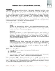
Figure 20: Estimating a reference arrival time of
40 ms at a vertical depth of 4 m
Figure 19: Implementation of the LLSR technique on
the relative arrival times illustrated in Figure 18
The LLSR technique is implemented by enabling check box Enable Linear Least Squares
Regression as outlined in Figure 3. The LLSR option also provides for DST arrival time
estimates. Figure 20 shows the output of the LLSR technique when processing the relative
arrival times outlined in Figure 18 and a reference arrival time and depth of 40 ms and 3.7 m,
respectively. As is shown in Figure 20, the depth interval of 6.7 m to 7.7 m does not have an
associated LLSR interval velocity estimate due to the fact that there is not an interval arrival time
estimate between 7.7 m and 8.7 m available.
Version 11.1.0 Page 13