Identification of dry and rainy periods using telecommunication ...
Identification of dry and rainy periods using telecommunication ...
Identification of dry and rainy periods using telecommunication ...

Create successful ePaper yourself
Turn your PDF publications into a flip-book with our unique Google optimized e-Paper software.
12 nd International Conference on Urban Drainage, Porto Alegre/Brazil, 10-15 September 2011<br />
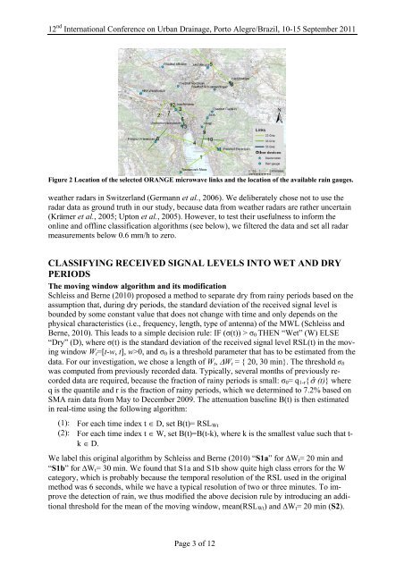
Figure 2 Location <strong>of</strong> the selected ORANGE microwave links <strong>and</strong> the location <strong>of</strong> the available rain gauges.<br />
weather radars in Switzerl<strong>and</strong> (Germann et al., 2006). We deliberately chose not to use the<br />
radar data as ground truth in our study, because data from weather radars are rather uncertain<br />
(Krämer et al., 2005; Upton et al., 2005). However, to test their usefulness to inform the<br />
online <strong>and</strong> <strong>of</strong>fline classification algorithms (see below), we filtered the data <strong>and</strong> set all radar<br />
measurements below 0.6 mm/h to zero.<br />
CLASSIFYING RECEIVED SIGNAL LEVELS INTO WET AND DRY<br />
PERIODS<br />
The moving window algorithm <strong>and</strong> its modification<br />
Schleiss <strong>and</strong> Berne (2010) proposed a method to separate <strong>dry</strong> from <strong>rainy</strong> <strong>periods</strong> based on the<br />
assumption that, during <strong>dry</strong> <strong>periods</strong>, the st<strong>and</strong>ard deviation <strong>of</strong> the received signal level is<br />
bounded by some constant value that does not change with time <strong>and</strong> only depends on the<br />
physical characteristics (i.e., frequency, length, type <strong>of</strong> antenna) <strong>of</strong> the MWL (Schleiss <strong>and</strong><br />
Berne, 2010). This leads to a simple decision rule: IF (σ(t)) > σ0 THEN “Wet” (W) ELSE<br />
“Dry” (D), where σ(t) is the st<strong>and</strong>ard deviation <strong>of</strong> the received signal level RSL(t) in the moving<br />
window Wt=[t-w, t], w>0, <strong>and</strong> σ0 is a threshold parameter that has to be estimated from the<br />
data. For our investigation, we chose a length <strong>of</strong> Wt, �Wt = { 20, 30 min}. The threshold σ0<br />
was computed from previously recorded data. Typically, several months <strong>of</strong> previously recorded<br />
data are required, because the fraction <strong>of</strong> <strong>rainy</strong> <strong>periods</strong> is small: σ0= q1-r{�ˆ (t)} where<br />
q is the quantile <strong>and</strong> r is the fraction <strong>of</strong> <strong>rainy</strong> <strong>periods</strong>, which we determined to 7.2% based on<br />
SMA rain data from May to December 2009. The attenuation baseline B(t) is then estimated<br />
in real-time <strong>using</strong> the following algorithm:<br />
(1): For each time index t � D, set B(t)= RSLWt<br />
(2): For each time index t � W, set B(t)=B(t-k), where k is the smallest value such that tk<br />
� D.<br />
We label this original algorithm by Schleiss <strong>and</strong> Berne (2010) “S1a” for �Wt= 20 min <strong>and</strong><br />
“S1b” for �Wt= 30 min. We found that S1a <strong>and</strong> S1b show quite high class errors for the W<br />
category, which is probably because the temporal resolution <strong>of</strong> the RSL used in the original<br />
method was 6 seconds, while we have a typical resolution <strong>of</strong> two or three minutes. To improve<br />
the detection <strong>of</strong> rain, we thus modified the above decision rule by introducing an additional<br />
threshold for the mean <strong>of</strong> the moving window, mean(RSLWt) <strong>and</strong> �Wt= 20 min (S2).<br />
Page 3 <strong>of</strong> 12