Identification of dry and rainy periods using telecommunication ...

More documents

Recommendations

Info

12 nd International Conference on Urban Drainage, Porto Alegre/Brazil, 10-15 September 2011 � � RSL(t) Figure 3 (Left) A simple classification tree with categories D and W based on the attributes RSL(t), σ(t), min(RSLWt), max(RSLWt) for a backward-looking moving window of length �Wt= 20 min. (Right) Illustration of different moving windows to construct the attributes for a case of RSL(t). Online versions of algorithms only use past data, i.e. backward-looking windows. An observation is classified as D, if i) the attribute RSL(t)� 39.81 [dBm] (�), ii) RSL(t)� 39.81 AND σ(t)� 0.3202 AND max(RSL(t))< -40.81(�), etc. Regressive classification trees and random forests The aim of a regressive classification tree is to predict a classification for a “case” based on its attributes (also: “variables”) (Breiman et al., 1984) (Figure 3, left). Here, we classify an observation RSL(t) based on attributes computed from past (online) or both past and future (offline) data (e.g., σ(t), min(RSLWt), etc.) (Figure 3, right). We used the rpart package in the statistical computing language R, which maximizes the mean decrease in the Gini-index (GI) (Gini, 1921) at every split. To every end-node a classification (W or D) is assigned, when the splitting stops. This occurs by default, when a maximum of 20 observations at every node is reached (Atkinson, 2000). A random forest basically consists of many regressive trees, it again relies on a training-set with in total m classified cases. Each tree of the forest is then constructed using a different bootstrap sample, which is drawn with replacement from the original data (Breiman, 2001). The criteria for building the classification forest are the same as for the single classification tree. After the construction of the random forest, each new observation is classified by all trees of the forest, where each tree give a votes and the final category is assigned based on the majority of the votes. As the sum of all decreases in GI over the whole tree for an attribute (e.g., min(RSLWt)) gives an estimate of its importance, the mean decrease in GI (�Gini) is a measure of the sensitivity of the classification to this attribute (Breiman, 2001). While we used rpart for the classification tree, the R package randomForest was used for the construction of random forests to analyze the MWL data. For the offline random-forest algorithm, we calculated the following attributes from forwardbackward-looking windows (Figure 3, right) (the online versions only relied on past data) with �Wt= {15, 30, 120 min}: i) RSL, ii) standard deviation (std), iii) slope of a fitted regression line (slope) and autocorrelation (lag=1) (autocor) (all relative), iv) min(RSL) (min), v) max(RSL) (max), vi and vii) the 10%- and the 90%-Quantile (q10, q90; only for �Wt= 120min) (all absolute), viii) the last rain intensity obtained by the weather radar (RTS_past) and a binary variable (0 or 1) depicting whether it had rained in the previous 10 - 40 min (rain_10_40_past) (information on past rainfall). Our expectation was that information on past precipitation could improve the classification. Intrinsic MWL variables, such as the cross-correlation between the two communication channels were also calculated, but finally not used in the classification, because it often resulted in zero standard variation in the intervals, for which the correlation coefficient is not defined. We constructed various random forests based on different attributes [in brackets] as online (ON) or offline version: RF1 [all attributes], RF2 [same as RF1, ON], RF3 [all-{RTS_past, rain_10_40_past}], RF4 [same as RF3, ON]. RF5 [{RSL, min}], RF6 [same as RF5, ON] consider only the most informative RSL (t) Page 4 of 12 time (t)
12 nd International Conference on Urban Drainage, Porto Alegre/Brazil, 10-15 September 2011 attributes, which we selected based on a high �Gini value. A table with the list of all used variables for RF1-RF6 is provided in Table A2. As the moving window algorithm repeatedly misclassified small rain amounts (see below), we introduced the additional category “light rain” (L) (D: 0, Light: 0.6, W> 0.6 [mm/h]). For training, we compiled sets of 1000 dry and 1000 rainy cases, randomly sampled out of the desired analysis period. Although this does not correspond to the observed distribution of dry and wet periods, it improves the detection of wet periods, which are more relevant in our application. 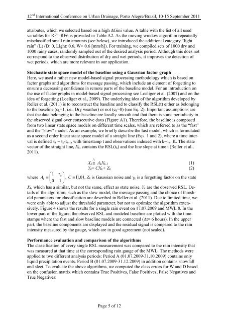Stochastic state space model of the baseline using a Gaussian factor graph Here, we used a rather new model-based signal processing methodology which is based on factor graphs and algorithms for message passing, which include an element of forgetting to ensure a decreasing confidence in remote parts of the baseline model. For an introduction on the use of factor graphs in model-based signal processing see Loeliger et al. (2007) and on the idea of forgetting (Loeliger et al., 2009). The underlying idea of the algorithm developed by Reller et al. (2011) is to reconstruct the baseline and to classify the RSL(t) either as belonging to the baseline (ck=1, i.e., Dry weather) or not (ck=0) (see Eq. 2). Important assumptions are that the data belonging to the baseline are locally smooth and that there is some periodicity in the observed signal over consecutive days (Figure A1). Therefore, the baseline is composed from two linear state space models on different time scales, which are referred to as the “fast" and the “slow" model. As an example, we briefly describe the fast model, which is formulated as a second order linear state space model of a straight line (Eqs. 1 and 2), where a time interval is defined �k = tk-tk-1, with timestamp t and observations indexed with k=1,..K. The state vector of the straight line, Xk, contains the RSL(tk) and the line slope at time t (Reller et al., 2011). � k Xk � AkXk-1 (1) Yk= CXk+ Zk (2) where �� 1 � k � Ak � �� , C � �1, 0�, Zk is Gaussian noise and �k is a forgetting factor on the state �0 1 � Xk, which has a similar, but not the same, effect as state noise. Yk are the observed RSL. Details of the algorithm, such as the slow model, the message passing and the choice of threshold parameters for classification are described in Reller et al. (2011). Due to limited time, we were only able to adjust the threshold parameter, but not to optimize the algorithm extensively. Figure 4 shows the results for a single rain event on 17.07.2009 and MWL 8. In the lower part of the figure, the observed RSL and modeled baseline are plotted with the timestamps where the fast and slow baseline models are connected (�t= 6 hours). In the upper part, the baseline components are displayed and the residual signal is compared to the rain intensity measured by the gauge, which are in good agreement (not scaled). Performance evaluation and comparison of the algorithms The classification of every single RSL measurement was compared to the rain intensity that was measured at that time at the corresponding rain gauge of the MWL. The methods were applied to two different analysis periods: Period A (01.07.2009-31.10.2009) contains only liquid precipitation events. Period B (01.07.2009-31.12.2009) in addition contains snowfall and sleet. To evaluate the above algorithms, we computed the class errors for W and D based on the confusion matrix which contains True Positives, False Positives, False Negatives and True Negatives: Page 5 of 12
Page 1 and 2: 12 nd International Conference on U
Page 3: 12 nd International Conference on U

Identification of dry and rainy periods using telecommunication ...

You also want an ePaper? Increase the reach of your titles

Delete template?

Save as template?