Identification of dry and rainy periods using telecommunication ...

12 nd International Conference on Urban Drainage, Porto Alegre/Brazil, 10-15 September 2011
class error for S1a and S1b increased to approximately 45% (coarse quantization: 75%). In
contrast, the wet class error for S2 only increased to 20 % (coarse quantization: 30%). As expected,
the dry class error did not experience important changes.
Regressive classification trees and random forests
Similar to the above algorithms, we developed individual classifiers for the 14 MWL based
on Random forests and the various attributes computed from period A data. As described
above, we classified dry (D) and rainy periods, split into light (L) and strong (W). The direct
comparison with S1-S2 shows rather favourable results for the random forest algorithms RF1-
RF6, because less than 5% of all rainy cases {L,W} were misclassified as dry (results not
shown). We found that the mean class errors for RF1- RF6 (averaged over all 14 links) for
class W were about 20%, with 30-50% errors for L, light rains, which means that many light
rains are wrongly classified as strong and vice versa. Also, the online algorithms perform
competitively against the offline algorithm, because the class error for W is very similar and
errors for the two other classes only increase slightly (e.g., D: RF1/RF2 = 19.9%/22.2%). For
period B, the class errors (averaged over all links and over RF1-RF6) showed an increase of
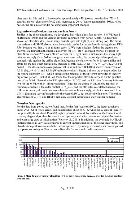
9.9 % (D), 3.9 % (L) and 8.5 % (W) (absolute values). Figure 6 shows the average �Gini for
the offline algorithm RF1, which indicates the potential of the different attributes to identify
dry or wet periods. First of all, we found that the important attributes depend on the quantization
of the MWL. Second, min(RSL) (for �Wt= {15,30}) and the RSL itself are very informative
for the MWL with 0.1 dBm resolution. Third, for the coarse MWL, the by far most informative
attribute is the radar rainfall (RTS_past) and the attributes calculated based on the
RSL unfortunately do not contain much information. Interestingly, attributes computed from
�Wt=120min are very informative for the coarse MWL, but not for the fine ones. The online
algorithms (RF2, RF4 and RF6) which only use past information show similar patterns.
Gaussian factor graphs
For the data from period A, we found that, for the fine (coarse) MWL, the factor graph produces
2% (7%) of type I errors, and misclassifies about 35% (32%) of the W class (Figure 7).
For period B, this is about 1% (5%) higher (absolute values). Nevertheless, the Factor Graph
is a very elegant algorithm, because it can cope very well with pronounced signal fluctuations
and even large gaps of missing data (Reller et al., 2011). In addition, the available MATLAB
implementation is very fast compared to current implementations of the other algorithms. The
classification performance could be further optimized by tuning, eventually also accompanied
by a post-processing to filter out unrealistically frequent and small rain events.
�Gini
180
160
140
120
100
80
60
40
20
0
min15_fut
min30_past
min15_past
min30_fut
RSL
RTS_past
min120_past
std120_past
std30_past
min120_fut
std30_fut
std120_fut
max15_fut
q10_120_fut
q10_120_past
std15_past
std15_fut
max15_past
autocor120_past
slope30_fut
Page 7 of 12
slope120_fut
slope30_past
max30_fut
autocor120_fut
slope120_past
max30_past
slope15_past
0.1 dB-Links
1 dB-Links
slope15_fut
q90_120_past
rain_10_40_past
autocor30_past
autocor30_fut
max120_fut
max120_past
autocor15_past
autocor15_fut
Figure 6 Mean Gini-decrease for algorithm RF1. �Gini is the average decrease over ten 0.1 dBm and four
1.0 dBm links.