Stockwell-Why Use the S-Transform.pdf - Bitbucket
Stockwell-Why Use the S-Transform.pdf - Bitbucket
Stockwell-Why Use the S-Transform.pdf - Bitbucket

Create successful ePaper yourself
Turn your PDF publications into a flip-book with our unique Google optimized e-Paper software.
Fields Institute Communications<br />
Volume 00, 0000<br />
<strong>Why</strong> use <strong>the</strong> S-<strong>Transform</strong>?<br />
R.G. <strong>Stockwell</strong><br />
Northwest Research Associates, Colorado Research Associates Division,3380 Mitchell Lane,<br />
Boulder Colorado USA 80301<br />
Abstract. The S-transform (ST) is a time-frequency representation<br />
known for its local spectral phase properties. A key feature of <strong>the</strong> Stransform<br />
is that it uniquely combines a frequency dependent resolution<br />
of <strong>the</strong> time-frequency space with absolutely referenced local phase information.<br />
This allows one to define <strong>the</strong> meaning of phase in a local<br />
spectrum setting, and results in many advantageous characteristics. It<br />
also exhibits a frequency invariant amplitude response, in contrast to<br />
<strong>the</strong> wavelet transform.<br />
This manuscript outlines <strong>the</strong> derivation of both <strong>the</strong> S-transform<br />
and <strong>the</strong> efficient Discrete Orthonormal S-transform and gives a detailed<br />
description of <strong>the</strong> implementation of <strong>the</strong> algorithms. The arbitrary sampling<br />
of <strong>the</strong> time-frequency space is illustrated and <strong>the</strong> direct connection<br />
between <strong>the</strong> S-transform, <strong>the</strong> Discrete Orthonormal S-transform, and<br />
<strong>the</strong> Fourier transform is described.<br />
Illustrations of <strong>the</strong> properties of <strong>the</strong> S-transform approach are given<br />
and a comparisons to wavelet transform is performed. The S-transform<br />
is shown to have absolutely referenced phase information, a quality that<br />
<strong>the</strong> continuous wavelet transform is lacking. In addition, <strong>the</strong> S-transform<br />
is shown to have a frequency invariant amplitude response in contrast<br />
to <strong>the</strong> continuous wavelet transform which attenuates high frequency<br />
signals relative to <strong>the</strong> low frequency signals.<br />
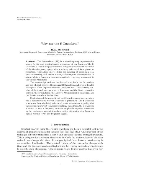
1 Introduction<br />
Spectral analysis using <strong>the</strong> Fourier transform has been a powerful tool in <strong>the</strong><br />
analysis of geophysical data (for instance [55], [56], [57], etc.). One drawback of <strong>the</strong><br />
technique of Fourier transforms is that it only produces <strong>the</strong> time-averaged spectrum.<br />
This is adequate for stationary time series in which <strong>the</strong> characteristics of <strong>the</strong> time<br />
series do not change with time. In <strong>the</strong> geophysical data, however, stationarity is<br />
an unrealized idealization. The spectral content of <strong>the</strong> time series changes with<br />
time, and <strong>the</strong> time-averaged amplitudes found by Fourier methods are inadequate<br />
to describe such phenomena. Thus in recent years, Fourier analysis has given way<br />
1991 Ma<strong>the</strong>matics Subject Classification. Primary ; Secondary.<br />
Supported by National Science Foundation Grant ATM-0350680.<br />
1<br />
c○0000 American Ma<strong>the</strong>matical Society
2 R.G. <strong>Stockwell</strong><br />
to more advanced representations known as joint time-frequency representations or<br />
TFRs.<br />
The S-transform (ST) [22] has found application in a range of fields. It is similar<br />
to a continuous wavelet transform in having progressive resolution but unlike <strong>the</strong><br />
wavelet transform, <strong>the</strong> S-transform retains absolutely referenced phase information<br />
and has a frequency invariant amplitude response. Absolutely referenced phase information<br />
means that <strong>the</strong> phase information given by <strong>the</strong> S-transform refers to <strong>the</strong><br />
argument of <strong>the</strong> cosinusoid at zero time (which is <strong>the</strong> same meaning of phase given<br />
by <strong>the</strong> Fourier transform). The S-transform defines what local phase means in an<br />
intuitive way, at a peak in local spectral amplitude (indicating a quasimonochromatic<br />
signal), as well as off peak, where <strong>the</strong> rate of change of <strong>the</strong> phase leads to a<br />
channel Instantaneous Frequency analysis. The S-transform not only estimates <strong>the</strong><br />
local power spectrum, but also <strong>the</strong> local phase spectrum. It is also applicable to<br />
<strong>the</strong> general complex valued time series.<br />
The role of phase in wavelet analysis is not as well understood as it is for<br />
<strong>the</strong> Fourier transform, especially for orthonormal wavelet representations. Current<br />
complex wavelets such as complex Daubechies wavelets [16], dual tree complex<br />
wavelets [17, 18, 19], and complex Shannon Wavelets [20] do not have a direct<br />
relationship to <strong>the</strong> Fourier transform.<br />
2 The Fourier <strong>Transform</strong><br />
It is often useful to think of <strong>the</strong> time series as a single vector in an N-dimensional<br />
vector space. The basis vectors of this time series in <strong>the</strong> time domain are <strong>the</strong> vectors<br />
(1,0,0,...,0), (0,1,0,...,0) and so on. The action of <strong>the</strong> Fourier transform is simply a<br />
change of basis on <strong>the</strong> time series, from <strong>the</strong>se delta function basis vectors (time domain),<br />
to sinusoidal basis vectors (frequency domain). The time series itself, which<br />
is a defined single vector in this N-dimensional vector space, remains unchanged.<br />
One of <strong>the</strong> reasons that <strong>the</strong> Fourier transform is ubiquitous in <strong>the</strong> analysis of<br />
geophysical phenomena is that <strong>the</strong> sinusoidal basis functions are <strong>the</strong> solution to <strong>the</strong><br />
ma<strong>the</strong>matical equations describing a small perturbation of a physical system about<br />
a stable equilibrium, and thus provides a suitable framework for studying such<br />
phenomena. Also a number of <strong>the</strong>oretical predictions concerning <strong>the</strong> evolution<br />
of such systems is easily couched in terms of Fourier <strong>the</strong>ory. Thus changing <strong>the</strong><br />
representation of <strong>the</strong> time series may present <strong>the</strong> information contained in <strong>the</strong> time<br />
series in a more easily assimilated form.<br />
The spectrum H(f) ofatimeseriesh(t) is given by standard Fourier analysis<br />
as [59]:<br />
� ∞<br />
H(f) = h(t)e −ı2πft dt (2.1)<br />
−∞<br />
and its inverse relationship is:<br />
� ∞<br />
h(t) = H(f)e ı2πft df (2.2)<br />
−∞<br />
where <strong>the</strong> units of t and f are such that <strong>the</strong> product is dimensionless.<br />
In dealing with a discrete time series of N points with a sampling interval of T ,<br />
<strong>the</strong> discrete Fourier transform (DFT) is used (where k =0...N−1andm =0...N−1)<br />
H<br />
�<br />
n<br />
�<br />
=<br />
NT<br />
1<br />
N−1 �<br />
N<br />
k=0<br />
ı2πnk −<br />
h [kT] e N (2.3)
<strong>Why</strong> use <strong>the</strong> S-<strong>Transform</strong>? 3<br />
Figure 1 a) Sample 256 point time series of an linearly increasing fre-<br />
quency chirp. The function is h(t) =sin( 2π<br />
20<br />
t 2<br />
256 2 ). b) Sample time series<br />
of similar to (1a), except here <strong>the</strong> frequency chirp is linearly decreasing.<br />
c,d ) Amplitude Spectra. e,f) Phase spectra.<br />
and its inverse relationship is:<br />
h [kT] =<br />
N−1 �<br />
n=0<br />
�<br />
n<br />
�<br />
H e<br />
NT<br />
ı2πnk<br />
N (2.4)<br />
The Fourier transform is limited in that, although it can determine <strong>the</strong> spectral<br />
components of a time series, it is lacking in information on when <strong>the</strong>se components<br />
occurred.<br />
2.1 A Motivating Example. A weakness in <strong>the</strong> Fourier transform representation<br />
of data is that <strong>the</strong> temporal information is not readily apparent; it is<br />
obscured in <strong>the</strong> phase spectrum of <strong>the</strong> Fourier transform. Very different data, with<br />
very different underlying physics, can have similar power spectra as shown in Figure<br />
1 with a simple chirp function (a sinusoid whose frequency increases (plot a) or<br />
decreases (plot b) linearly in time).<br />
As shown in Figure 1c,d <strong>the</strong> amplitude spectra are identical for both time series,<br />
indicating that <strong>the</strong>re is no information about when <strong>the</strong> different frequencies existed<br />
in <strong>the</strong> time series. The time-local information is hidden in <strong>the</strong> value of <strong>the</strong> phases<br />
of <strong>the</strong> spectrum in Figure 1e,f, but this information is not readily accessible. From<br />
this point of view, <strong>the</strong> purpose of time-frequency representations is to unfold this<br />
temporal information into a more easily digestible form.<br />
3 The S-transform<br />
The S-transform produces a time-frequency representation of a time series. It<br />
uniquely combines a frequency dependent resolution with simultaneously localizing<br />
<strong>the</strong> real and imaginary spectra. It was first published in 1996 [22], and since has<br />
seen several interesting applications (see [69] and references <strong>the</strong>rein).
4 R.G. <strong>Stockwell</strong><br />
The continuous S-transform [22] of a function h(t) is<br />
� ∞<br />
S(τ,f)=<br />
−∞<br />
h(t) |f|<br />
√ 2π e − (τ−t)2 f 2<br />
2 e −i2πft dt. (3.1)<br />
A “voice” S(τ,f0) is defined as a one dimensional function of time for a constant<br />
frequency f0, which shows how <strong>the</strong> amplitude and phase for this exact frequency<br />
changes over time. A “local spectrum” S(τ0,f) is a one dimensional function of<br />
frequency for a constant time t0.<br />
<strong>Why</strong> <strong>the</strong> Gaussian Window? The Gaussian window is chosen for several reasons:<br />
1) it uniquely minimizes <strong>the</strong> quadratic time-frequency moment about a timefrequency<br />
point [70], 2) it is symmetric in time and frequency - <strong>the</strong> Fourier transform<br />
of a Gaussian is a Gaussian, 3) <strong>the</strong>re are no sidelobes in a Gaussian function (a<br />
local maxima in <strong>the</strong> absolute value of <strong>the</strong> S-transform is not an artifact). However,<br />
as is <strong>the</strong> case with Power Spectral Estimation, any desired window or apodizing<br />
function may be employed.<br />
3.1 Derivation of S-<strong>Transform</strong> from STFT:. If <strong>the</strong> time series h(t) is<br />
windowed (or multiplied point by point) with a window function g(t) <strong>the</strong>n <strong>the</strong><br />
resulting spectrum is<br />
� ∞<br />
H(f) = h(t)g(t)e −ı2πft dt (3.2)<br />
−∞<br />
The S-transform can be found by first defining a particular window function, a<br />
normalized Gaussian<br />
g(t) = 1<br />
σ √ t2<br />
e− 2σ<br />
2π 2 (3.3)<br />
and <strong>the</strong>n allowing <strong>the</strong> Gaussian to be a function of translation τ and dilation (or<br />
window width) σ.<br />
S ∗ � ∞<br />
1<br />
(τ,f,σ) = h(t)<br />
−∞ σ √ (t−τ)2<br />
e− 2σ<br />
2π 2 e −ı2πft dt (3.4)<br />
which, with a particular value of σ, is similar in definition to <strong>the</strong> STFT. This is a<br />
special case of <strong>the</strong> Multiresolution Fourier transform. Because this is a function of<br />
three independent variables, it is impractical as a tool for analysis. Simplification<br />
can be achieved by adding <strong>the</strong> constraint restricting <strong>the</strong> width of <strong>the</strong> window σ to<br />
be proportional to <strong>the</strong> period (or inverse of <strong>the</strong> frequency)<br />
σ(f) = 1<br />
(3.5)<br />
| f |<br />
Thus one has <strong>the</strong> S-transform of equation 3.1.<br />
3.2 ST as a Convolution. The S-transform can be written as a convolution<br />
of two functions over <strong>the</strong> variable t<br />
� ∞<br />
S(τ,f)= p(t, f)g(τ − t, f)dt (3.6)<br />
or<br />
where<br />
−∞<br />
S(τ,f)=p(τ,f) ∗ g(τ,f) (3.7)<br />
p(τ,f)=h(τ)e −ı2πfτ<br />
(3.8)
<strong>Why</strong> use <strong>the</strong> S-<strong>Transform</strong>? 5<br />
and<br />
g(τ,f)=<br />
| f |<br />
√ 2π e − τ2 f 2<br />
2 (3.9)<br />
Let B(α, f) be <strong>the</strong> Fourier transform (from τ to α) of <strong>the</strong> S-transform S(τ,f).<br />
By <strong>the</strong> convolution <strong>the</strong>orem <strong>the</strong> convolution in <strong>the</strong> τ (time) domain becomes a<br />
multiplication in <strong>the</strong> α (frequency) domain:<br />
B(α, f) =P (α, f)G(α, f) (3.10)<br />
(Likewise, P (α, f) andG(α, f) are <strong>the</strong> Fourier transform of p(τ,f) andg(τ,f).)<br />
Explicitly,<br />
B(α, f) =H(α + f)e − 2π2 α 2<br />
f 2 (3.11)<br />
where H(α + f) is <strong>the</strong> Fourier transform of (3.8), and <strong>the</strong> exponential term is<br />
<strong>the</strong> Fourier transform of <strong>the</strong> Gaussian function (3.9). Thus <strong>the</strong> S-transform is <strong>the</strong><br />
inverse Fourier transform (from α to τ) of <strong>the</strong> above equation (for f �= 0).<br />
� ∞<br />
S(τ,f)=<br />
−∞<br />
H(α + f)e − 2π2 α 2<br />
f 2 e ı2πατ dα (3.12)<br />
The exponential function in Eq. (3.12) is <strong>the</strong> frequency dependent localizing window<br />
andiscalled<strong>the</strong>Voice Gaussian. This window is centered around <strong>the</strong> zero frequency<br />
and thus plays <strong>the</strong> role of a low pass filter for each particular voice. This is in<br />
contrast to a wavelet or band pass filtered approach to calculating voices of a timefrequency<br />
representation.<br />
3.3 Derivation of <strong>the</strong> S-transform from <strong>the</strong> Wavelet <strong>Transform</strong>. The<br />
following derivation demonstrates <strong>the</strong> relationship between <strong>the</strong> S-transform and <strong>the</strong><br />
continuous wavelet transform. The continuous wavelet transform can be defined as<br />
a series of correlations of <strong>the</strong> time series with a function called a wavelet:<br />
� ∞<br />
W (τ,d) = h(t)<br />
−∞<br />
1 t − τ<br />
√ ψ( )dt (3.13)<br />
d d<br />
The S-transform of a function h(t) can be defined as a CWT with a specific mo<strong>the</strong>r<br />
wavelet multiplied by a correction factor and by replacing dilation d with <strong>the</strong> inverse<br />
of frequency f:<br />
�<br />
f<br />
S(τ,f)=<br />
2π e−i2πfτ W (τ,f) (3.14)<br />
where <strong>the</strong> mo<strong>the</strong>r wavelet is defined as<br />
ψ((t − τ)f) =e − (t−τ)2 f 2<br />
2 −ı2πf(t−τ )<br />
e<br />
(3.15)<br />
The wavelet in (3.15) does not satisfy <strong>the</strong> admissibility condition of having a<br />
zero mean, and <strong>the</strong>refore (3.14) is not strictly a CWT. Writing out (3.14) explicitly<br />
gives <strong>the</strong> S-transform as seen in (3.1).<br />
There are two vital terms in <strong>the</strong> S-transform definition: 1) <strong>the</strong> phase function<br />
e −ı2πft and 2) <strong>the</strong> normalization |f|<br />
√ 2π . The phase function, resulting from application<br />
of <strong>the</strong> phase factor in Eq. (3.14) deserves fur<strong>the</strong>r discussion. It is in fact<br />
a phase correction of <strong>the</strong> definition of <strong>the</strong> Wavelet transform. It eliminates <strong>the</strong><br />
concept of “wavelet analysis” by separating <strong>the</strong> mo<strong>the</strong>r wavelet into two parts, <strong>the</strong><br />
slowly varying envelope (<strong>the</strong> Gaussian function) which localizes in time, and <strong>the</strong><br />
oscillatory exponential kernel e −ı2πft which selects <strong>the</strong> frequency being localized. It<br />
is <strong>the</strong> time localizing Gaussian that is translated while <strong>the</strong> oscillatory exponential
6 R.G. <strong>Stockwell</strong><br />
kernel remains stationary. By not translating <strong>the</strong> oscillatory exponential kernel, <strong>the</strong><br />
S-transform localizes <strong>the</strong> real and <strong>the</strong> imaginary components of <strong>the</strong> spectrum independently,<br />
localizing <strong>the</strong> phase spectrum as well as <strong>the</strong> amplitude spectrum. This is<br />
referred to as absolutely referenced phase information. Absolutely referenced phase<br />
means that <strong>the</strong> phase information given by <strong>the</strong> S-transform is always referenced to<br />
time t = 0, which is also true for <strong>the</strong> phase given by <strong>the</strong> Fourier transform. This is<br />
true for each S-transform sample of <strong>the</strong> time-frequency space. The normalization<br />
factor also deserves fur<strong>the</strong>r discussion. It normalizes <strong>the</strong> time domain localizing<br />
window (<strong>the</strong> Gaussian function) to have unit area. In doing this, <strong>the</strong> amplitude of<br />
<strong>the</strong> S-transform has <strong>the</strong> same meaning as <strong>the</strong> amplitude of <strong>the</strong> Fourier transform.<br />
This provides a frequency invariant amplitude response in contrast to <strong>the</strong> Wavelet<br />
approach. The term “frequency invariant amplitude response” means that for a<br />
sinusoid with an amplitude A0 (h(t) = A0cos(2πft)), <strong>the</strong> S-transform returns an<br />
amplitude A0 regardless of <strong>the</strong> frequency f.<br />
3.4 Linearity and <strong>the</strong> Effect of Noise. The S-transform is a linear operation<br />
on <strong>the</strong> time series h(t). This is important for <strong>the</strong> case of additive noise in which<br />
one can model <strong>the</strong> data as data(t) =signal(t)+noise(t) and thus <strong>the</strong> operation of<br />
<strong>the</strong> S-transform leads to<br />
S{data} = S{signal} + S{noise} (3.16)<br />
This is an advantage over <strong>the</strong> bilinear class of TFRs (such as Cohen’s Class [7] )<br />
where one finds<br />
TFR{data} = TFR{signal} + TFR{noise}<br />
+ 2∗TFR{signal}∗TFR{noise} (3.17)<br />
3.5 Discrete ST. In <strong>the</strong> discrete case, <strong>the</strong>re are computational advantages to<br />
using <strong>the</strong> equivalent frequency domain definition of <strong>the</strong> S-transform (where H[ n<br />
NT ]<br />
is <strong>the</strong> Fourier transform of <strong>the</strong> N-point time series h[kT])<br />
S[jT, n<br />
NT ]=<br />
N/2−1 �<br />
m=−N/2<br />
m + n<br />
H[<br />
NT ]e− 2π2 m 2<br />
n2 e i2πmj<br />
N , n �= 0 (3.18)<br />
and for <strong>the</strong> n = 0 voice, it is equal to <strong>the</strong> constant defined as<br />
S[jT,0] = 1<br />
N−1 �<br />
h[kT] (3.19)<br />
N<br />
where j, m and n =0,1,..., N − 1. The sampling of <strong>the</strong> S-transform is such that<br />
S[jT, n<br />
NT ] has a point at each time sample and at each Fourier frequency sample.<br />
Similar to a STFT and CWT, this is redundant.<br />
3.6 Discrete Inverse S-transform. The discrete inverse of <strong>the</strong> S-transform<br />
is performed through <strong>the</strong> intermediate step of computing <strong>the</strong> discrete Fourier transform.<br />
Summing <strong>the</strong> S-transform matrix along <strong>the</strong> voices (rows) gives (n �= 0)<br />
N−1 �<br />
j=0<br />
S[ n<br />
NT ,jT]=<br />
N−1 �<br />
N/2−1 �<br />
k=0<br />
m + n<br />
H[<br />
NT<br />
j=0 m=−N/2<br />
]e− 2π2 m2 n2 e i2πmj<br />
N (3.20)
<strong>Why</strong> use <strong>the</strong> S-<strong>Transform</strong>? 7<br />
Reordering <strong>the</strong> sequence of summation, we have<br />
N−1 �<br />
j=0<br />
S[ n<br />
NT ,jT]=<br />
N/2−1 �<br />
m=−N/2<br />
�<br />
m + n<br />
H[<br />
NT ]e− 2π2 m2 n2 N−1<br />
e<br />
j=0<br />
i2πmj<br />
N (3.21)<br />
By <strong>the</strong> orthogonal property, <strong>the</strong> sum over j is zero unless m = zero in which case<br />
it is equal to N. Thus <strong>the</strong> average of <strong>the</strong> voices of S(n/NT, jT )is<br />
N−1 �<br />
j=0<br />
S[ n<br />
NT ,jT]=<br />
N/2−1 �<br />
m=−N/2<br />
m + n<br />
Nδm,0H[<br />
NT ]e− 2π2 m 2<br />
n2 . (3.22)<br />
N−1<br />
1 �<br />
S[<br />
N<br />
j=0<br />
n<br />
n<br />
,jT]=H[ ]. (3.23)<br />
NT NT<br />
Therefore <strong>the</strong> discrete inverse of <strong>the</strong> S-transform is (∀n):<br />
h[kT] = 1<br />
N<br />
N−1 �<br />
n=0<br />
⎧<br />
⎨N−1<br />
�<br />
S[<br />
⎩<br />
n<br />
NT ,jT]<br />
⎫<br />
⎬<br />
⎭<br />
j=0<br />
e i2πnk<br />
N . (3.24)<br />
3.7 Implementation of S-<strong>Transform</strong> algorithm. Figure2showsaschematic<br />
representation of <strong>the</strong> implementation of <strong>the</strong> Discrete S-transform. The first step<br />
of <strong>the</strong> ST algorithm is to calculate <strong>the</strong> Fourier transform of <strong>the</strong> N-point time series.<br />
One <strong>the</strong>n shifts <strong>the</strong> spectrum so that <strong>the</strong> voice frequency becomes <strong>the</strong> zero<br />
frequency. This shift is <strong>the</strong> phase correction of Eq. 3.14. One <strong>the</strong>n multiplies <strong>the</strong><br />
spectrum with <strong>the</strong> N-point voice Gaussian function to select <strong>the</strong> frequency range.<br />
The N-point inverse Fourier transform is applied to this product to populate <strong>the</strong><br />
voice of <strong>the</strong> ST as indicated by <strong>the</strong> arrow labeled IFFT (each voice will have Npoints).<br />
This procedure (applying <strong>the</strong> window and performing <strong>the</strong> inverse FT) is<br />
repeated until all <strong>the</strong> voices are populated. By employing <strong>the</strong> fast Fourier transform<br />
algorithm, <strong>the</strong> calculation of <strong>the</strong> voices is extremely efficient.<br />
This has very strong parallels to <strong>the</strong> implementation of <strong>the</strong> DOST shown below.<br />
3.8 The S-transform and <strong>the</strong> Analytic Signal. For a simple signal, that<br />
of a sinusoid with a constant frequency,<br />
h(t) =exp(ı2πfot) (3.25)<br />
Vakman [60] gives <strong>the</strong> following definition for <strong>the</strong> Instantaneous Frequency:<br />
IF(t) = 1 ∂<br />
arg(t) (3.26)<br />
ı2π ∂t<br />
where <strong>the</strong> argument (or phase) of this function is<br />
arg(t) =ı2πfot. (3.27)<br />
and <strong>the</strong> frequency is f = fo = arg<br />
ı2πt .<br />
To calculate <strong>the</strong> Instantaneous Frequency function <strong>the</strong> original time series has<br />
to be transformed into <strong>the</strong> following form:<br />
h(t) =A(t)exp(Arg(t)) (3.28)<br />
and <strong>the</strong>n <strong>the</strong> Arg(t) function must be extracted by use of <strong>the</strong> arctan function.<br />
If <strong>the</strong> time series is real-valued, however, <strong>the</strong>n <strong>the</strong> phase has no meaning (being<br />
identically equal to zero).
8 R.G. <strong>Stockwell</strong><br />
Figure 2 Schematic of <strong>the</strong> S-transform algorithm. Top left plot shows<br />
<strong>the</strong> S-transform amplitude for positive frequencies. The top right plot<br />
shows <strong>the</strong> Fourier transform amplitudes with <strong>the</strong> frequencies on <strong>the</strong> yaxis<br />
in order to line up with <strong>the</strong> frequency axis of <strong>the</strong> ST plot. The<br />
bottom left plot shows <strong>the</strong> time series with <strong>the</strong> time axis lined up with<br />
<strong>the</strong> ST plot.<br />
Following Vakman [60] <strong>the</strong> Hilbert transform is used to extend <strong>the</strong> real-valued<br />
time series into a complex time series. The phase is <strong>the</strong>n <strong>the</strong> usual definition of<br />
phase for a complex function. The Hilbert transform of a function h(t) is[61]<br />
X(τ) = 1<br />
π<br />
�<br />
h(t)<br />
dt (3.29)<br />
τ − t<br />
and <strong>the</strong> inverse is<br />
h(t) = 1<br />
�<br />
X(τ)<br />
dτ<br />
π τ − t<br />
(3.30)<br />
The Analytic Signal of a real function is defined as:<br />
AS{h(t)} = h(t)+iX(t) (3.31)<br />
Therefore <strong>the</strong> Instantaneous Frequency (in radians) is <strong>the</strong> defined as [60]:<br />
IF(t) = ∂<br />
∂t arctan(ℑ[AS(t)] ) (3.32)<br />
ℜ[AS(t)]<br />
or<br />
IF(t) = ∂<br />
∂t arctan(X(t) ) (3.33)<br />
h(t)<br />
It can be shown that <strong>the</strong> Analytic Signal is closely related to <strong>the</strong> S-transform.<br />
The S-transform is a band pass filtered analytic signal of <strong>the</strong> original time series
<strong>Why</strong> use <strong>the</strong> S-<strong>Transform</strong>? 9<br />
h(t). Starting from Eq. 3.12, one can shift <strong>the</strong> spectrum by replacing α with<br />
κ = α + f, and treating f as an arbitrary parameter<br />
� ∞<br />
S(τ,f)=<br />
−∞<br />
H(κ)e − 2π2 (κ−f) 2<br />
f 2 e ı2πατ dκ (3.34)<br />
The negative frequencies are removed from this time series (if f is positive). Thus<br />
any voice of <strong>the</strong> S-transform corresponds to a band pass filtered Analytic Signal of<br />
<strong>the</strong>originaltimeseries.<br />
3.8.1 Instantaneous Frequency and <strong>the</strong> Nyquist Frequency. Since phase is defined<br />
as:<br />
Φ(z) = arctan( ℑ[z]<br />
) (3.35)<br />
ℜ[z]<br />
<strong>the</strong>re is a 2π ambiguity in <strong>the</strong> value for each value of phase resulting from <strong>the</strong> use<br />
of <strong>the</strong> arctan function. Thus when one samples <strong>the</strong> phase of <strong>the</strong> Analytic Signal,<br />
<strong>the</strong> phase function must be unrolled. For any change with a magnitude greater<br />
than π, one must add or subtract multiples of 2π so that <strong>the</strong> change is smaller than<br />
π. Since <strong>the</strong> time series is discretely sampled with a sampling interval of T ,<strong>the</strong><br />
maximum rate-of-change of <strong>the</strong> phase is π over one time unit and is <strong>the</strong> Nyquist<br />
radial frequency<br />
fMAX = π<br />
(3.36)<br />
T<br />
3.8.2 Channel Instantaneous Frequency. The use of Instantaneous Frequency<br />
in a local spectral representation was introduced for <strong>the</strong> S-transform [22], and independently<br />
was employed by Nelson [50] to study nonstationary multicomponent<br />
FM signals. Gardner and Magnasco [51] also used band-pass filtered Instantaneous<br />
Frequency analysis for <strong>the</strong> analysis of sound.<br />
The S-transform approach (including <strong>the</strong> DOST described below) provides an<br />
extension of Instantaneous Frequency to broadband signals. The voice for a particular<br />
frequency ν1 can be written as<br />
S(τ,ν1) =A(τ,ν1)e iΦ(τ,ν1) . (3.37)<br />
One may use <strong>the</strong> phase in Eq. 3.37 to determine <strong>the</strong> “local” Instantaneous Frequency<br />
similar to that defined by Bracewell [52].<br />
GIF (τ,ν1) = 1 ∂<br />
2π ∂τ {2πν1τ +Φ(τ,ν1)} (3.38)<br />
Thus <strong>the</strong> absolutely referenced phase information leads to a generalization of <strong>the</strong><br />
Instantaneous Frequency to broadband signals.<br />
The measure of Instantaneous Frequency is not quantized to <strong>the</strong> sampled frequencies,<br />
and thus can achieve arbitrarily high accuracy. In essence, <strong>the</strong> application<br />
of <strong>the</strong> Generalized Instantaneous Frequency can be utilized as a local peak-finding<br />
algorithm. Again, <strong>the</strong>re are ringing effects and wrap around effects that are familiar<br />
in discrete Fourier transform analysis.<br />
3.9 Cross ST Analysis. Because of <strong>the</strong> ST phase characteristic, it can be<br />
employed in a cross spectrum analysis in a local manner. Consider two time series<br />
measured by two devices separated by a known distance. Let a sinusoidal wave<br />
propagate through <strong>the</strong> field of view of both devices. What will be seen by <strong>the</strong>se<br />
devices is a sinusoid, but with a time shift between <strong>the</strong> two time series. Since <strong>the</strong><br />
ST localizes spectral components in time, <strong>the</strong> cross correlation of specific events<br />
on two spatially separated STs will give <strong>the</strong> phase difference and hence <strong>the</strong> phase
10 R.G. <strong>Stockwell</strong><br />
velocity can be derived with knowledge of <strong>the</strong> frequency and <strong>the</strong> distance between<br />
measurements.<br />
The amplitude of <strong>the</strong> CrossST indicates coincident signals. The phase of <strong>the</strong><br />
CrossST at local maxima indicates <strong>the</strong> phase lag (or phase difference) between those<br />
two coincident signals. The Cross ST of two time series h(t) andg(t) is defined as:<br />
CrossST(τ,f)=Sh(τ,f) {Sg(τ,f)} ∗<br />
(3.39)<br />
where <strong>the</strong> phase of <strong>the</strong> CrossST is given by<br />
arg(CrossST )=Φ(τ,f)h − Φ(τ,f)g<br />
(3.40)<br />
3.9.1 The S-transform Shift Theorem. As written above, <strong>the</strong> S-transform is<br />
defined as<br />
S(τ,f)= f<br />
√ 2π<br />
�<br />
h(t)e − (t−τ)2 f 2<br />
2 e −ı2πft dt (3.41)<br />
If one translates <strong>the</strong> time series by an amount r, one can study <strong>the</strong> effect on <strong>the</strong><br />
S-transform by making a change of variables t → (k − r)<br />
S(τ,f)= f<br />
�<br />
√ h(k − r)e<br />
2π<br />
− ((k−r)−τ)2 f 2<br />
2 e −ı2πf(k−r) dk (3.42)<br />
Rearranging <strong>the</strong> equation gives<br />
S(τ,f)= f<br />
��<br />
√ h(k − r)e<br />
2π<br />
− (k−(τ+r))2 f 2<br />
2 e −ı2πfk �<br />
dk e ı2πfr<br />
(3.43)<br />
Making ano<strong>the</strong>r change of variables, τ → (z − r)<br />
S(z − r, f )e −ı2πfr = f<br />
�<br />
√ h(k − r)e<br />
2π<br />
− (k−z)2 f 2<br />
2 e −ı2πfk dk (3.44)<br />
Thus <strong>the</strong> S-transform Shift Theorem states that if<br />
h(t) ⇔ S(τ,f) (3.45)<br />
<strong>the</strong>n<br />
h(t − r) ⇔ S(τ − r, f )e −ı2πfr<br />
(3.46)<br />
3.9.2 Time shift of a monochromatic signal. Starting with equation 3.12<br />
�<br />
S(τ,f)=<br />
H(α + f)e − 2π2 α 2<br />
f 2 e ı2πατ dα (3.47)<br />
<strong>the</strong> S-transform of a sinusoidal function h(t)<br />
h(t) =e ı2πwt<br />
with a spectrum<br />
(3.48)<br />
H(α) = 1<br />
δ(α − w)<br />
2<br />
(3.49)<br />
is<br />
�<br />
S(τ,f)= δ(α + f − w)e − 2π2 α 2<br />
f2 e ı2πατ or<br />
dα (3.50)<br />
S(τ,f)= 1<br />
(f−w)2<br />
(<br />
e−<br />
2 f<br />
2π )2 e ı2π(f−w)τ<br />
If one introduces a constant phase shift into <strong>the</strong> sinusoid,<br />
(3.51)<br />
g(t) =h(t)e iΦ = e ı2πwt+ıΦ<br />
(3.52)
<strong>Why</strong> use <strong>the</strong> S-<strong>Transform</strong>? 11<br />
Figure 3 Illustration of <strong>the</strong> CrossST of two time series.<br />
with a resulting spectrum<br />
H(α) = 1<br />
δ(α − w)eıΦ<br />
2<br />
this results in a phase shift of <strong>the</strong> S-transform<br />
S{g(t)} (τ,f) = 1<br />
2<br />
(f−w)2<br />
(<br />
e− f<br />
2π )2 e ı2π(f−w)τ e ıΦ<br />
(3.53)<br />
(3.54)<br />
Thus if one performs a localized cross spectral S-transform analysis by multiplying<br />
<strong>the</strong> ST of h(t) with <strong>the</strong> complex conjugate of <strong>the</strong> ST of g(t)<br />
S(τ,f) {h(t)} · � �∗ S(τ,f) {g(t)}<br />
= 1 f 2<br />
2π<br />
2<br />
The phase of <strong>the</strong> Cross ST is<br />
e− (f−w)2<br />
ı2π(f−w)τ 1<br />
e<br />
2 e<br />
(f−w) 2<br />
f 2<br />
2π e −ı2π(f−w)τ e −ıΦ<br />
(3.55)<br />
Phase {ShS ∗ g } (τ,f) = −Φ (3.56)<br />
This can be used to find a localized time lag between <strong>the</strong> two time series as a<br />
function of t and f. This result is true for <strong>the</strong> general time series.<br />
In Figure 3, two syn<strong>the</strong>tic time series are created with three distinct sinusoidal<br />
components. A low frequency component for <strong>the</strong> first half, a mid frequency component<br />
for <strong>the</strong> second half, and a high frequency burst signal at <strong>the</strong> one quarter<br />
mark. For each of <strong>the</strong> two signals, <strong>the</strong> low frequency signal is in phase (i.e. both<br />
cosine function). The mid frequency is out of phase (<strong>the</strong> first signal is a cosine function,<br />
<strong>the</strong> second signal is a sine function). The high frequency burst is in phase,<br />
but temporally translated in <strong>the</strong> second functions such that <strong>the</strong>re is only a brief<br />
overlap.
12 R.G. <strong>Stockwell</strong><br />
Figure 4 Illustration of <strong>the</strong> CrossST of two time series. The phase voice<br />
for each of <strong>the</strong> three components is shown, and <strong>the</strong> correct phase lag for<br />
each is indicated.<br />
In Figure 4, individual ST phase voices of <strong>the</strong> CrossST are shown. The ST phase<br />
voice for <strong>the</strong> low frequency component correctly shows a zero phase lag between<br />
<strong>the</strong> two time series for <strong>the</strong> first half. The amplitude is negligible for this voice in<br />
<strong>the</strong> second half. For <strong>the</strong> medium frequency voice, <strong>the</strong> ST phase voice correctly<br />
shows <strong>the</strong> π/2 phase lag between <strong>the</strong> two time series for this component (<strong>the</strong> first<br />
time series had a cos(), and <strong>the</strong> second time series had a sin() for this component).<br />
For <strong>the</strong> high frequency burst, <strong>the</strong> ST phase voice in <strong>the</strong> region of overlap between<br />
time = 200 and time = 250 shows <strong>the</strong> correct phase lag of 0 radians. O<strong>the</strong>r times<br />
(indicated by <strong>the</strong> grey trace) have a negligible amplitude, and <strong>the</strong>refore <strong>the</strong> phase<br />
is meaningless.<br />
3.10 Co-ST and Quadrature ST. There is still more information that can<br />
be gleaned from <strong>the</strong> CrossST analysis. Because of <strong>the</strong> phase characteristics of <strong>the</strong><br />
ST, one can utilize <strong>the</strong> cross ST function to analyze <strong>the</strong> in-phase and out-of-phase<br />
components in time-frequency space.<br />
As with classical co-spectrum analysis, <strong>the</strong> real part of <strong>the</strong> cross ST function<br />
gives <strong>the</strong> in-phase components of <strong>the</strong> local spectra. The imaginary part of <strong>the</strong> cross<br />
ST function gives <strong>the</strong> in-quadrature components.<br />
Figure 5a shows <strong>the</strong> ST amplitude of <strong>the</strong> first signal. Figure 5b shows <strong>the</strong><br />
ST amplitude of <strong>the</strong> second signal. The ST amplitudes of <strong>the</strong> two signals are<br />
very similar, except for <strong>the</strong> temporal translation of <strong>the</strong> high frequency component.<br />
Figure 5c,d,e show <strong>the</strong> Cross ST, <strong>the</strong> Co-ST and <strong>the</strong> Quadrature ST amplitudes<br />
respectively. In <strong>the</strong> Cross ST plot, all three components appear. However <strong>the</strong> high<br />
frequency component only occurs for a brief time, indicating <strong>the</strong> overlap between<br />
<strong>the</strong> two time-shifted signals. In <strong>the</strong> co-ST, only <strong>the</strong> features that are in phase are<br />
present - those being <strong>the</strong> low frequency component and <strong>the</strong> high frequency burst.<br />
The middle frequency (which is out of phase) does not appear. In <strong>the</strong> quadrature ST<br />
plot only <strong>the</strong> out-of-phase signals appear, which is <strong>the</strong> middle frequency component.<br />
3.11 Analysis of a Complex Time Series. Spectral analysis of a two component<br />
time series has been performed [53] on data such as <strong>the</strong> horizontal wind field
<strong>Why</strong> use <strong>the</strong> S-<strong>Transform</strong>? 13<br />
Figure 5 Illustration of <strong>the</strong> co-ST and <strong>the</strong> Quadrature ST.<br />
[u(t),v(t)] by constructing a one dimensional complex-valued time series as follows<br />
U[t] =u[t]+ıv[t] =A(t)e ıωt<br />
(3.57)<br />
where u[t] is <strong>the</strong> zonal wind (positive eastward), v[t] is <strong>the</strong> meridional wind (positive<br />
northward), ı = √ −1, ω is <strong>the</strong> radial frequency of rotation, and A(t) is <strong>the</strong> amplitude<br />
function. The Fourier transform of a complex valued time series requires both<br />
<strong>the</strong> positive and negative frequencies to completely characterize <strong>the</strong> wind. Such<br />
“rotary spectral” analysis will decompose <strong>the</strong> wind motions into circular (clockwise<br />
and counter-clockwise) components.<br />
As with <strong>the</strong> Fourier transform, both <strong>the</strong> S-transform and <strong>the</strong> DOST can be applied<br />
to a 2 component vector time series such as <strong>the</strong> horizontal wind field [u(t),v(t)]<br />
by constructing a one dimensional complex valued time series as in Eq. 3.57.<br />
By looking at <strong>the</strong> phase difference between <strong>the</strong> positive and negative frequencies<br />
it is possible to infer complete information of <strong>the</strong> generalized elliptical motion,<br />
including <strong>the</strong> sense of rotation, <strong>the</strong> major and minor axes, and ellipticity [54]. A<br />
syn<strong>the</strong>tic time series illustrating this effect is shown in Figure 6. The complex time<br />
series depicts a counter-clockwise rotating surface wind vector, with an amplitude<br />
that starts small, grows in time, <strong>the</strong>n decays. The time series was constructed in
14 R.G. <strong>Stockwell</strong><br />
Figure 6 (a) A two component time series, (analogous to a horizontal<br />
wind measurement for instance) that initially increases in amplitude,<br />
<strong>the</strong>n decreases in amplitude. Additionally, <strong>the</strong> wind is rotating counterclockwise.<br />
(b) The S-transform amplitude. The changing amplitude can<br />
be seen. The counter-clockwise motion can be seen in that <strong>the</strong> positive<br />
frequency component is larger than <strong>the</strong> negative frequency component.<br />
<strong>the</strong> form of Eq. 3.57 as follows U[t] =80cos(2πt24.4/128) + ı60 sin(2πt24.4/128)<br />
where t =0, 1...127 and <strong>the</strong> amplitude is varied by multiplying <strong>the</strong> time series<br />
with a hanning window. The amplitude of <strong>the</strong> S-transform of this time series is<br />
shown in Figure 6b. The white background denotes regions of negligible energy,<br />
and filled regions correspond to large amplitudes. The peak amplitude occurs at<br />
f =24/128 and t = 64. Because this amplitude is larger than its mirror in <strong>the</strong><br />
negative frequencies (f = −24/128 and t = 64), this represents a counter-clockwise<br />
oscillation. If <strong>the</strong> negative frequency is larger, <strong>the</strong>n rotation is clockwise.<br />
4 The Discrete Orthonormal S-transform (DOST)<br />
There are several reasons to desire an orthonormal time-frequency version of<br />
<strong>the</strong> S-transform. An orthonormal transformation takes an N-point time series to an<br />
N-point time-frequency representation, thus achieving maximum efficiency. Also,<br />
each point of <strong>the</strong> result is independent from any o<strong>the</strong>r point. The transformation<br />
matrix is orthogonal, meaning that <strong>the</strong> inverse matrix is equal to <strong>the</strong> complex<br />
conjugate transpose. By being an orthonormal transformation, <strong>the</strong> vector norm<br />
is preserved. Thus a Parseval <strong>the</strong>orem applies, stating that <strong>the</strong> norm of <strong>the</strong> time<br />
series equals <strong>the</strong> norm of <strong>the</strong> DOST.<br />
The efficient representation of <strong>the</strong> S-transform can be defined as <strong>the</strong> inner<br />
products between a time series h[kT] and <strong>the</strong> basis functions defined as a function<br />
of [kT], with <strong>the</strong> parameters ν (a frequency variable indicative of <strong>the</strong> center of a<br />
frequency band and analogous to <strong>the</strong> “voice” of <strong>the</strong> S-transform), β (indicating <strong>the</strong>
<strong>Why</strong> use <strong>the</strong> S-<strong>Transform</strong>? 15<br />
frequency resolution), and τ (a time variable indicating <strong>the</strong> time localization).<br />
S{h[kT]} = S(τT, ν<br />
NT )=<br />
k=N−1 �<br />
h[kT]S [ν,β,τ ][kT] (4.1)<br />
4.1 Derivation of <strong>the</strong> basis functions. By extending filter bank <strong>the</strong>ory, in<br />
combination with <strong>the</strong> unique phase correction of <strong>the</strong> S-transform, <strong>the</strong> time domain<br />
basis functions for <strong>the</strong> S-transform are developed. Within a frequency band (i.e. a<br />
particular voice), several orthogonal basis functions are formed by a linear combination<br />
of <strong>the</strong> Fourier basis functions in that frequency band. There are β components<br />
in this operation. Thus β basis functions can be derived by applying <strong>the</strong> appropriate<br />
phase functions to <strong>the</strong> components (where each of <strong>the</strong> β basis functions is<br />
indexed by τ =0, 1, ...β −1). The key to creating orthogonal functions is <strong>the</strong> careful<br />
selection of <strong>the</strong> frequency shift applied to <strong>the</strong> Fourier basis functions. This action<br />
is <strong>the</strong> analog of <strong>the</strong> “phase correction” of <strong>the</strong> S-transform. This is where <strong>the</strong> absolutely<br />
referenced phase information originates, and it is what distinguishes <strong>the</strong>se<br />
basis functions from wavelets. It is also <strong>the</strong> inclusion of this additional operation<br />
that is distinct from a simple filtering operation. One should note, <strong>the</strong> voices of <strong>the</strong><br />
DOST cannot be created by a filtering operation of <strong>the</strong> original time series.<br />
The basis functions can be derived by starting with a partitioning of <strong>the</strong> spectrum<br />
(a simple restricted sum of complex-valued Fourier basis functions) defined<br />
in <strong>the</strong> time domain (function of [kT]), centered at frequency ν with a bandwidth<br />
of β and applying <strong>the</strong> appropriate phase and frequency shifts:<br />
S(kT) [ν,β,τ ] =<br />
1<br />
√ β<br />
f=ν+ β<br />
2 −1<br />
�<br />
f=ν− β<br />
2<br />
k=0<br />
exp(i2π k<br />
τ<br />
N<br />
f)exp(−i2π f)exp(−i2π τT) (4.2)<br />
N β 2NT<br />
where 1<br />
√ β is a normalization factor to insure orthonormality of <strong>the</strong> basis functions.<br />
Thus <strong>the</strong> basis function for <strong>the</strong> Discrete Orthonormal S-transform (DOST) of<br />
voice frequency ν, bandwidth β, and time index τ can be written as:<br />
S(kT) [ν,β,τ ] = e−iπτ<br />
√ β<br />
Application of <strong>the</strong> identity<br />
f=ν+ β<br />
2 −1<br />
�<br />
f=ν− β<br />
2<br />
exp(i2π( k τ<br />
− )f) (4.3)<br />
N β<br />
c + cx + ... + cx n−1 = c(1 − xn )<br />
1 − x<br />
to Eq. 4.3 leads to <strong>the</strong> basis functions S [ν,β,τ ][kT] for <strong>the</strong> general case<br />
S [ν,β,τ ][kT] = ie−iπτ<br />
√ β<br />
k τ β 1<br />
−i2π( N − β )(ν− 2 − 2 ) k τ β 1<br />
−i2π(<br />
− e N − β )(ν+ 2 − 2 ) }<br />
{e<br />
The limit of <strong>the</strong> basis function as k<br />
N<br />
lim<br />
k τ<br />
N → β<br />
→ τ<br />
β<br />
2sin[π( k τ<br />
N − β )]<br />
is well behaved and equal to:<br />
S(kT) [ν,β,τ ] = � βe iπτ<br />
(4.4)<br />
(4.5)<br />
(4.6)
16 R.G. <strong>Stockwell</strong><br />
At this point, <strong>the</strong> sampling of <strong>the</strong> time-frequency space has not yet been determined.<br />
Rules must be applied to <strong>the</strong> sampling of <strong>the</strong> time-frequency space to<br />
ensure orthogonality. These rules are as follows:<br />
• Rule 1: τ =0, 1, ···β − 1.<br />
• Rule 2: ν and β must be selected such that each Fourier frequency sample<br />
is used once and only once.<br />
Implicit in this definition is <strong>the</strong> phase correction of <strong>the</strong> S-transform that distinguishes<br />
it from <strong>the</strong> wavelet or filter bank approach. For each voice, <strong>the</strong>re are one<br />
or more local time samples (τ), this number being equal to β (see Rule 1) thus <strong>the</strong><br />
wider <strong>the</strong> frequency resolution (large β), <strong>the</strong> greater <strong>the</strong> time resolution (large τ)<br />
which implicitly shows <strong>the</strong> Uncertainty Principle.<br />
Distinct from a wavelet function, <strong>the</strong>se basis functions have no vanishing moments<br />
(in fact <strong>the</strong> functions are normalized to unit area). These basis functions are<br />
not translations of a single function, and <strong>the</strong>y are not self-similar.<br />
One advantage of this method is that one can directly calculate any voice, without<br />
having to iterate through a series of intermediate steps. Also, <strong>the</strong>re is no filter<br />
design involved nor any upsampling or downsampling algorithms required. Ano<strong>the</strong>r<br />
advantage is that it allows one to directly apply <strong>the</strong> ideas of Power Spectrum Estimation,<br />
such as applying windows and apodizing functions, to <strong>the</strong> analysis of <strong>the</strong><br />
local spectrum of a time series.<br />
Note that in a departure from filter bank <strong>the</strong>ory, <strong>the</strong> sum is centered on <strong>the</strong><br />
voice frequency ν. In o<strong>the</strong>r words, a frequency translation has been applied. The<br />
operation of calculating <strong>the</strong> inner product of a time series with this basis function<br />
not equivalent to a simple filtering operation (in <strong>the</strong> asymptotically simple case of<br />
<strong>the</strong> time series consisting of an oscillating sinusoid, <strong>the</strong> resulting voice will be a constant,<br />
in amplitude and phase, for each time sample). This frequency shift is vital<br />
when <strong>the</strong> characteristic of absolutely referenced phase information (and cross local<br />
spectrum analysis and generalized instantaneous frequency) is described, and is <strong>the</strong><br />
distinguishing difference between <strong>the</strong> S-transform approach, and <strong>the</strong> wavelet/filter<br />
bank approach. This shift in frequency is <strong>the</strong> key feature of <strong>the</strong> original S-transform.<br />
In Eq 11 of [22], <strong>the</strong> “n ′′ voice S[jT, n<br />
NT<br />
] has <strong>the</strong> same frequency translation applied<br />
by <strong>the</strong> shift of <strong>the</strong> spectrum H[(m + n)/N T ]by“n” which centers <strong>the</strong> spectrum<br />
around <strong>the</strong> n frequency in Eq. 3.18. It is precisely this property of <strong>the</strong> basis<br />
functions that provides absolutely referenced phase information, and it is also this<br />
property that implies that <strong>the</strong> basis functions are not self-similar.<br />
It is easy to show that <strong>the</strong> basis functions are indeed orthonormal and have<br />
compact support in frequency. They are not compactly supported in time, but <strong>the</strong>y<br />
are local. The property of “compact support” refers to a particular transform. An<br />
orthonormal wavelet does not have compact support under a Fourier transform. By<br />
<strong>the</strong> Uncertainty Principle, one cannot have a compactly supported function which<br />
has a compact Fourier transform. These basis functions are compact in frequency,<br />
and also local in time, while maintaining orthogonality. The requirement is that<br />
<strong>the</strong> ν and β values are chosen such that <strong>the</strong> bandwidths do not overlap, and that<br />
all discrete frequencies are sampled.<br />
The fundamental difference between <strong>the</strong> discrete orthonormal wavelet transform<br />
(DWT) and <strong>the</strong> DOST is in <strong>the</strong> absolutely referenced phase information [69].<br />
The phase of a voice of <strong>the</strong> DOST has <strong>the</strong> same meaning as <strong>the</strong> phase of a component<br />
of <strong>the</strong> Fourier transform.
<strong>Why</strong> use <strong>the</strong> S-<strong>Transform</strong>? 17<br />
As is well known from Fourier <strong>the</strong>ory, <strong>the</strong> translation in time of <strong>the</strong> wavelet (or<br />
any function) corresponds to a phase modulation in <strong>the</strong> Fourier spectral domain.<br />
Thus, wavelet voices have a phase modulation applied to <strong>the</strong>m in <strong>the</strong> spectral<br />
domain. This is not true for <strong>the</strong> DOST as <strong>the</strong>re is no direct translation applied<br />
to <strong>the</strong> basis function to produce o<strong>the</strong>r basis functions. It is this characteristic of<br />
self-similarity that force this phase modulation (and <strong>the</strong>refore <strong>the</strong> lack of absolutely<br />
referenced phase) on all wavelet transforms.<br />
The fundamental idea of a wavelet transform is <strong>the</strong> decomposition of a signal<br />
into deformations of a mo<strong>the</strong>r wavelet. In <strong>the</strong> analysis of geophysical data, often<br />
<strong>the</strong> local characteristics of <strong>the</strong> phase of <strong>the</strong> signal can lead to great insight. In order<br />
to resolve <strong>the</strong> local phase properties, it is necessary to break <strong>the</strong> analyzing wavelets<br />
from <strong>the</strong> mo<strong>the</strong>r wavelet, and impart an absolutely referenced phase to <strong>the</strong> basis<br />
functions. This break separates <strong>the</strong> time-localizing windowing function, from <strong>the</strong><br />
frequency-localizing modulation. As <strong>the</strong> time-localizing window translates in time,<br />
it is essential for this formalism that <strong>the</strong> frequency modulation does not translate<br />
in time, which <strong>the</strong>n forbids <strong>the</strong> possibility of self-similar basis functions. One can<br />
ei<strong>the</strong>r have a self-similar basis (wavelets), or an absolutely referenced phase basis<br />
(DOST).<br />
4.2 Orthonormal basis functions with Octave Sampling. In order to<br />
compare <strong>the</strong> DOST with orthonormal wavelet transforms and with <strong>the</strong> S-transform,<br />
an octave sampling of <strong>the</strong> time-frequency domain is illustrated (following [69]).<br />
This has <strong>the</strong> property of progressive resolution that <strong>the</strong> S-transform shares. Octave<br />
sampling implies that <strong>the</strong> voice bandwidth doubles for each increasing voice (as<br />
sampling allows).<br />
By imposing specific rules on <strong>the</strong> basis functions (here octave sampling) it<br />
implies a strict definition for ν and β. By introducing a new variable p which<br />
corresponds to <strong>the</strong> octave number p =0, 1, 2, ··· ,log2(N) − 1 one can define all <strong>the</strong><br />
parameters (ν, β, τ) of equation 4.5 in terms of p as follows:<br />
For p>1, we have:<br />
p = 2, ..log2(N) − 1 (4.7)<br />
ν = 2 (p−1) +2 (p−2)<br />
(4.8)<br />
β = 2 (p−1)<br />
(4.9)<br />
τ = 0, 1,..2 (p−1) − 1 (4.10)<br />
For <strong>the</strong> case p =0,<strong>the</strong>nν =0andβ =1andτ =0. Alsowhenp =1,<strong>the</strong>nν =1<br />
and β =1andτ =0.<br />
Thus <strong>the</strong> DOST basis functions for octave sampling of a time series are given<br />
as follows (by application of 4.7, 4.8, 4.9 and 4.10 into 4.5):<br />
S [p,τ ][kT] = ie−iπτ {e<br />
√<br />
2 (p−1)/2<br />
k τ<br />
−i2π( N −<br />
2p−1 )(2p−1− 1<br />
2 ) k τ<br />
−i2π(<br />
− e N −<br />
2p−1 )(2p− 1<br />
2 ) }<br />
2sin[π( k τ<br />
N − 2p−1 )]<br />
(4.11)<br />
The application of <strong>the</strong> DOST with octave sampling for <strong>the</strong> case where N = 100<br />
is illustrated in Figures 7 and 8 [69]. In Figure 7, octave sampled DOST basis<br />
functions are shown for a specific DOST voice (p = 5 and <strong>the</strong>refore ν =24and<br />
bandwidth β = 16), for six different time samples (τ =5...10). These functions<br />
are not simple translations, as is most evident in a comparison of Figures 7d and<br />
Figure 7f.
18 R.G. <strong>Stockwell</strong><br />
Figure 7 Selected DOST basis functions of increasing time with octave<br />
sampling for N = 100. Note that <strong>the</strong> DOST functions are not<br />
translates of a single function.<br />
Figure 8 also shows six octave sampled DOST basis functions, but now <strong>the</strong><br />
order p varies (as does voice frequency ν and <strong>the</strong> bandwidth β). Thetimesampleτ<br />
is chosen simply to center <strong>the</strong> function. Again <strong>the</strong> lack of <strong>the</strong> self-similar property<br />
is evident. No basis function shown in Figure 8 is a dilation of any o<strong>the</strong>r basis<br />
function.<br />
While octave partitioning has <strong>the</strong> familiar frequency dependent resolution seen<br />
in <strong>the</strong> S-transform and wavelets, <strong>the</strong> formalism defined in Eq. 4.5 allows for any<br />
arbitrary sampling of <strong>the</strong> time-frequency space (similar to o<strong>the</strong>r frame based wavelet<br />
approaches). Often <strong>the</strong> resolution of <strong>the</strong> time-frequency space is dependent on <strong>the</strong><br />
source signal; a transient signal will have a broad spectral signature regardless of<br />
sampling. Also, while it may be inferred that <strong>the</strong> above algorithm assumes that<br />
<strong>the</strong> number of points N is a power of two, that is not a strict requirement for<br />
octave sampling (as shown in Figures 7 and 8). The octave sampling scheme can<br />
be applied to any arbitrary length time series by starting at <strong>the</strong> Nyquist frequency<br />
with<br />
β = truncate(float(truncate(N/2) + 1)/2) (4.12)<br />
and for each lower frequency partition, reducing <strong>the</strong> bandwidth as follows<br />
βnew = truncate(float(β +1)/2) (4.13)
<strong>Why</strong> use <strong>the</strong> S-<strong>Transform</strong>? 19<br />
Figure 8 Selected DOST basis functions of increasing voice frequency<br />
with octave sampling for N = 100. Each plot shows a basis<br />
function (solid line = real, dotted line = imaginary) from a different<br />
frequency range (i.e. different voice).<br />
For example, <strong>the</strong> octave sampling for N = 31 is {1,1,2,4,8,8,4,2,1} where <strong>the</strong> first element<br />
is <strong>the</strong> DC level, <strong>the</strong>n <strong>the</strong> next four β are <strong>the</strong> positive frequencies (increasing),<br />
and <strong>the</strong> last four β are <strong>the</strong> negative frequencies (decreasing).<br />
4.3 Implementation of <strong>the</strong> DOST. Similar to <strong>the</strong> S-transform, <strong>the</strong> implementation<br />
of <strong>the</strong> DOST is more efficiently calculated from <strong>the</strong> Fourier Spectrum<br />
of <strong>the</strong> time series. This is shown in Figure 9. The DOST begins with <strong>the</strong> DFT of<br />
<strong>the</strong> time series, indicated by <strong>the</strong> vertical list of frequency index numbers. This is<br />
partitioned into <strong>the</strong> frequency bands (ν) containing β points. The subspace inverse<br />
DFT (IDFT) is applied to to each partitioned frequency band. Note that this is<br />
not <strong>the</strong> N-point IDFT, but it is a β-point IDFT. This insures that β points are<br />
created in <strong>the</strong> voice, and that <strong>the</strong> decomposition is orthogonal.<br />
For certain purposes it is highly desirable to window and interpolate <strong>the</strong> DOST<br />
time-frequency representation and approach <strong>the</strong> more ample sampling of <strong>the</strong> Stransform.<br />
<strong>Use</strong> of windowing and interpolation allows one to build up a smoo<strong>the</strong>r<br />
and less sparse representation of <strong>the</strong> time-frequency space, and in <strong>the</strong> extreme case<br />
of “fully redundant” interpolation (i.e. where a time-frequency representation point<br />
is calculated for each time sample of <strong>the</strong> original time series and for each frequency<br />
sample of <strong>the</strong> Fourier Spectrum) <strong>the</strong>n one can recreate <strong>the</strong> action of <strong>the</strong> original
20 R.G. <strong>Stockwell</strong><br />
Figure 9 Schematic of <strong>the</strong> DOST algorithm.<br />
S-transform. The DOST forms <strong>the</strong> essential skeleton of <strong>the</strong> time-frequency plane,<br />
from which <strong>the</strong> fully redundant S-transform can be derived.<br />
Figure 10 shows a schematic of <strong>the</strong> implementation of <strong>the</strong> oversampled DOST,<br />
and <strong>the</strong> steps necessary to window and oversample <strong>the</strong> time frequency space in<br />
any arbitrary manner. In this figure, <strong>the</strong> brackets represent <strong>the</strong> application of an<br />
overlapping window functions. The choice of window function is arbitrary as with<br />
Fourier transform spectral analysis, and any window or apodizing function may be<br />
used.<br />
The oversampling of <strong>the</strong> time-frequency space is illustrated in Figure 11. A<br />
modulated sinusoid time series is shown in Figure 11a. The amplitude DOST is<br />
shown in Figure 11b, and <strong>the</strong> smooth redundant S-transform amplitude is shown<br />
in Figure 11e, with intermediate steps shown in Figure 11c and d. Thus, one can<br />
achieve any arbitrary level of compromise between efficient representation (DOST)<br />
and a smooth and redundant representation by arbitrary choice of oversampling<br />
and windowing. The application of windowing to <strong>the</strong> DOST is easily done when
<strong>Why</strong> use <strong>the</strong> S-<strong>Transform</strong>? 21<br />
Figure 10 Schematic of <strong>the</strong> oversampling of <strong>the</strong> time-frequency space<br />
for <strong>the</strong> DOST algorithm.<br />
one realizes that an implicit boxcar window is applied to <strong>the</strong> spectral partition in<br />
<strong>the</strong> implementation of <strong>the</strong> DOST algorithm. In fact, any window (or apodizing<br />
function) can be applied at that stage. This is called “voice windowing” and is<br />
analogous to <strong>the</strong> “voice Gaussian” of <strong>the</strong> S-transform [22]. If one applies such a<br />
window, and thus reduces one’s sensitivity at <strong>the</strong> edges of <strong>the</strong> frequency bands,<br />
<strong>the</strong>n it becomes desirable to interpolate and oversample in frequency. When a<br />
window is applied to <strong>the</strong> partitioned spectrum, one should expect this new band<br />
to be representative of frequencies ν ± bandwidth of window, ra<strong>the</strong>r than (in <strong>the</strong><br />
case of unwindowed DOST) ν ± β/2.<br />
If one wished to interpolate <strong>the</strong> DOST in time, this can be accomplished by<br />
widening <strong>the</strong> partitions in <strong>the</strong> frequency domain so that <strong>the</strong>y overlap (thus <strong>the</strong><br />
partitioned spectrum is <strong>the</strong>n extended to more higher and lower frequencies interpolating<br />
<strong>the</strong> time domain voice). As one goes to full interpolation in time (i.e. a<br />
sample at every time sample of <strong>the</strong> original time series) <strong>the</strong>n <strong>the</strong>re is no partitioning<br />
(each spectral partition is <strong>the</strong> original spectrum). Only <strong>the</strong> shift of <strong>the</strong> spectrum
22 R.G. <strong>Stockwell</strong><br />
Figure 11 Illustration of <strong>the</strong> progression from <strong>the</strong> efficient DOST timefrequency<br />
representation (b) to <strong>the</strong> redundant S-transform representation<br />
(e) by increasingly interpolated (and windowed) DOSTs. Only<br />
positive frequencies and <strong>the</strong> amplitudes are shown. The time series is<br />
h[t] =cos(2 ∗ π ∗ (204 + 6 ∗ 1024/(1 + t) ∗ cos(2 ∗ π ∗ 3 ∗ t/1024)) ∗ t/1024)<br />
where t =0, 1, 1023<br />
(centering <strong>the</strong> voice frequency ν) and <strong>the</strong> voice-windowing will differentiate different<br />
frequency ranges.<br />
The DOST has <strong>the</strong> following properties:<br />
• exact analytical definition of a basis for <strong>the</strong> S-transform.<br />
• an orthogonal time-frequency transform from which <strong>the</strong> Discrete Fourier<br />
transform can be derived as a special case.<br />
• an orthogonal time-frequency representation that collapses over <strong>the</strong> time<br />
variable to exactly give <strong>the</strong> Discrete Fourier transform spectrum.<br />
• absolutely referenced phase, thus giving meaning to <strong>the</strong> phase of an orthonormal<br />
time-frequency representation.
<strong>Why</strong> use <strong>the</strong> S-<strong>Transform</strong>? 23<br />
• <strong>the</strong> ability to directly compare <strong>the</strong> phase of two time series in a “localized<br />
cross spectral analysis”.<br />
• <strong>the</strong> ability to employ a channel “instantaneous frequency” to each voice of<br />
<strong>the</strong> DOST.<br />
• a general definition of a time-frequency representation to which one can<br />
apply any of <strong>the</strong> standard windows of power spectrum analysis in order to<br />
perform a localized power spectrum analysis.<br />
• introduction of <strong>the</strong> framework to arbitrarily oversample <strong>the</strong> orthogonal timefrequency<br />
representation on all <strong>the</strong> way to <strong>the</strong> redundant S-transform, and<br />
thus showing how one can perform time-frequency analysis of almost arbitrarily<br />
large geophysical data sets with any desired sampling of <strong>the</strong> timefrequency<br />
space.<br />
• The DOST can be extended in a straightforward method to higher dimensions<br />
for applications such as image processing, and volumetric data analysis,<br />
as has been done with <strong>the</strong> S-transform.<br />
It should be noted that all properties of <strong>the</strong> ST described in section 3 are<br />
shared with <strong>the</strong> DOST. They are merely different yet complementary strategies for<br />
sampling and smoothing of <strong>the</strong> time-frequency space.<br />
5 Wavelet <strong>Transform</strong><br />
The continuous Wavelet transform was introduced by Goupillaud, Grossmann,<br />
and Morlet in 1984 [11]. The basic philosophy is that any time series can be<br />
decomposed into a series of dilations and compressions of a mo<strong>the</strong>r wavelet denoted<br />
as w(t). The advantage of this view is that high frequencies can be localized to a<br />
smaller time interval than low frequencies, which is a property it shares with <strong>the</strong><br />
S-transform. The continuous wavelet transform (CWT) of h(t) is given by [14]:<br />
� ∞<br />
1 −<br />
F (a, b) =| a | 2 h(t)w<br />
−∞<br />
∗ t − b<br />
( )dt (5.1)<br />
a<br />
where <strong>the</strong> asterisk denotes <strong>the</strong> complex conjugate. Strictly, <strong>the</strong> continuous wavelet<br />
transform gives a representation in <strong>the</strong> state space of <strong>the</strong> scale factor (or dilation) a<br />
and translation b, but with <strong>the</strong> appropriate choice of wavelet w(t),itcanbeusedto<br />
measure <strong>the</strong> power spectrum locally. Certain restrictions are placed on <strong>the</strong> function<br />
w(t) in order to do a wavelet analysis. These are [66] (where W (f) is <strong>the</strong> Fourier<br />
transform of w(t)):<br />
• w(t) must be absolutely and square integrable<br />
�<br />
2 dt<br />
| w(t) | < ∞. (5.2)<br />
R |t|<br />
• W (f) mustbereal.<br />
• W (f) must be small around f =0.<br />
These conditions ensure that <strong>the</strong> wavelet has finite energy and is band limited.<br />
The Morlet wavelet [67] is often encountered in <strong>the</strong> literature. The Morlet wavelet<br />
function consists of a complex exponential modulated by a Gaussian envelope:<br />
π −1/4 s −1/2 exp[ikx/s]exp[−(x/s) 2 /2] (5.3)<br />
where s is <strong>the</strong> wavelet scale, k is a non-dimensional parameter, and x is <strong>the</strong> position<br />
[68]. The IDL routine WV CWT is used to calculate <strong>the</strong> CWT results in this<br />
manuscript.
24 R.G. <strong>Stockwell</strong><br />
The continuous wavelet transform only localizes <strong>the</strong> power spectrum as a function<br />
of time. It does not retain <strong>the</strong> absolutely referenced phase information that<br />
<strong>the</strong> S-transform contains and <strong>the</strong>refore is not directly invertible to <strong>the</strong> Fourier<br />
transform spectrum. Due to its frequency dependent normalization <strong>the</strong> CWT with<br />
Morlet wavelets diminishes <strong>the</strong> high frequency components of <strong>the</strong> time-frequency<br />
space.<br />
6 A Comparison of <strong>the</strong> S-transform and <strong>the</strong> Continuous Wavelet<br />
<strong>Transform</strong><br />
What distinguishes <strong>the</strong> S-transform from <strong>the</strong> many time-frequency representations<br />
available is that <strong>the</strong> S-transform uniquely combines three characteristics: 1)<br />
progressive resolution, 2) absolutely referenced phase information, and 3) frequency<br />
invariant amplitude response. Daubechies has stated that progressive resolution<br />
gives a fundamentally more sound time-frequency representation [12].<br />
The absolutely referenced phase of <strong>the</strong> S-transform is in contrast to a wavelet<br />
approach, where <strong>the</strong> phase of <strong>the</strong> wavelet transform is relative to <strong>the</strong> center (in<br />
time) of <strong>the</strong> analyzing wavelet. Thus as <strong>the</strong> wavelet translates, <strong>the</strong> reference point<br />
of <strong>the</strong> phase translates. This is called “locally referenced phase” to distinguish it<br />
from <strong>the</strong> phase properties of <strong>the</strong> S-transform.<br />
From one point of view, local spectral analysis is a generalization of <strong>the</strong> global<br />
Fourier Spectrum. In fact, since no record of observations is infinite, all discrete<br />
spectral analysis ever performed on measured data have been local (i.e. restricted<br />
to <strong>the</strong> time of observation). Thus <strong>the</strong>re must be a direct relationship between a<br />
local spectral representation and <strong>the</strong> global Fourier spectrum. This philosophy can<br />
be stated as <strong>the</strong> fundamental principle of S-transform analysis:<br />
The time average of <strong>the</strong> local spectral representation should result<br />
identically in <strong>the</strong> complex-valued global Fourier Spectrum.<br />
� ∞ �� ∞ �<br />
h(t) =<br />
S(τ,f)dτ e<br />
−∞ −∞<br />
ı2πft df (6.1)<br />
This shows that <strong>the</strong> S-transform can be thought of as a generalization of <strong>the</strong><br />
Fourier transform to nonstationary timeseries. A similar claim can not be made for<br />
<strong>the</strong> CWT. This leads to phase and amplitude values of <strong>the</strong> local spectrum that are<br />
obvious and meaningful. Consider a signal h(t) =Aexp(i2πfot + φ). The Fourier<br />
transform spectrum of this signal at <strong>the</strong> frequency fo would return <strong>the</strong> amplitude<br />
of A and <strong>the</strong> phase constant φ. In order to carry this understanding of phase into<br />
<strong>the</strong> realm of time-frequency representations and local spectra, it would require a<br />
transform that would return a voice (function of time) for <strong>the</strong> frequency fo that<br />
had a constant amplitude A and a constant phase φ. Such is <strong>the</strong> case with <strong>the</strong> Stransform,<br />
and thus it can be described as a generalization of <strong>the</strong> Fourier transform<br />
to <strong>the</strong> case of nonstationary signals.<br />
6.1 Frequency Sampling. The discrete Fourier transform has a very definite<br />
sampling of <strong>the</strong> frequencies, in order to be both complete and orthonormal (and<br />
thus provide a basis for <strong>the</strong> time series). The discrete ST has <strong>the</strong> identical sampling<br />
of <strong>the</strong> frequency space. It also has <strong>the</strong> same sampling of <strong>the</strong> time domain as <strong>the</strong><br />
original time series. Hence <strong>the</strong>re are N 2 points in <strong>the</strong> redundant ST representation.<br />
Conversely, <strong>the</strong> CWT has a loosely defined sampling of <strong>the</strong> TFR domain (Figure<br />
12). It is commonly employed with an octave scaling of <strong>the</strong> frequencies which
<strong>Why</strong> use <strong>the</strong> S-<strong>Transform</strong>? 25<br />
Figure 12 Frequency sampling histogram for <strong>the</strong> CWT and <strong>the</strong> ST<br />
(which is identical to <strong>the</strong> frequency sampling of <strong>the</strong> DFT). The ST is<br />
uniform in frequency, while <strong>the</strong> CWT oversamples <strong>the</strong> lower frequency<br />
region.<br />
Figure 13 Illustration of <strong>the</strong> extraction of a signal from <strong>the</strong> ST.<br />
provides an oversampled representation of <strong>the</strong> lowest frequencies, and undersamples<br />
(relative to <strong>the</strong> Fourier transform) <strong>the</strong> highest frequencies.<br />
6.2 Direct Signal Extraction. Because of <strong>the</strong> characteristics of <strong>the</strong> S-transform<br />
one can read off <strong>the</strong> amplitude A(t) = abs(S(t,f)), <strong>the</strong> frequency f, and <strong>the</strong> phase<br />
φ(t) = atan(real(S(t,f))) , imaginary(S(t,f))) for each time step from <strong>the</strong> S-transform
26 R.G. <strong>Stockwell</strong><br />
Figure 14 Illustration of <strong>the</strong> phase properties of <strong>the</strong> ST.<br />
and directly extract that signal by reproducing it in <strong>the</strong> time domain as follows:<br />
signal(t) =A(t)cos(2πf(t) ∗ t + φ(t)). (6.2)<br />
This direct extraction of a signal is due to <strong>the</strong> combination of absolutely referenced<br />
phase information and frequency invariant amplitude of <strong>the</strong> S-transform, and such<br />
direct extraction cannot be done with Wavelet methods. This shows that not only<br />
does <strong>the</strong> S-transform have a direct connection with <strong>the</strong> Fourier spectrum, it also<br />
has a direct connection with <strong>the</strong> original time series.<br />
For <strong>the</strong> example shown here in Figure 13 a chirp signal is combined with a<br />
noisy high frequency signal. The nearest neighbour maxima for <strong>the</strong> chirp signal are<br />
chosen for extraction, and <strong>the</strong> resulting chirp signal is cleanly extracted (Figure 13c<br />
and d).<br />
6.3 ST Phase vs CWT Phase. A peak in <strong>the</strong> ST is a region of stationary<br />
phase as can be seen by <strong>the</strong> definition for Generalized Instantaneous Frequency Eq.<br />
3.38. The stationary phase of <strong>the</strong> S-transform can be seen in <strong>the</strong> phase voices of<br />
Figure 14. This figure shows a particular voice for <strong>the</strong> signal shown in Figure 3<br />
for <strong>the</strong> mid frequency component. In <strong>the</strong> first plot, <strong>the</strong> phase of <strong>the</strong> CWT for that<br />
voice is shown, and it is rapidly varying through <strong>the</strong> full range of phase (from −π<br />
to π). In <strong>the</strong> second plot, <strong>the</strong> phase of <strong>the</strong> ST for <strong>the</strong> mid frequency component<br />
is shown. It is constant, and is equal to 0.4radians (which is <strong>the</strong> correct phase).<br />
In <strong>the</strong> third plot, <strong>the</strong> phase of local CWT spectrum is shown for time t =0. The<br />
amplitude of <strong>the</strong> local CWT spectrum is overplotted as a dotted line. The phase<br />
at <strong>the</strong> peak is not equal to <strong>the</strong> phase of <strong>the</strong> signal. In <strong>the</strong> fourth plot, <strong>the</strong> phase<br />
of <strong>the</strong> S-transform local spectra is shown for time t = 0, and <strong>the</strong> amplitude local<br />
spectrum is overplotted as a dotted line. The phase varies quite a bit for very low<br />
frequencies, but phase is meaningless when <strong>the</strong> amplitude is negligible (as shown<br />
by <strong>the</strong> dotted line). For <strong>the</strong> region where <strong>the</strong> amplitude has a significant value, <strong>the</strong>
<strong>Why</strong> use <strong>the</strong> S-<strong>Transform</strong>? 27<br />
Figure 15 (a) <strong>the</strong> ST amplitude of a cross chirp signal. (b) The phase<br />
of <strong>the</strong> ST for <strong>the</strong> cross chirp signal. The chirp is apparent in <strong>the</strong> phase<br />
due to <strong>the</strong> stationary phase of <strong>the</strong> ST at local maxima. At a peak in<br />
<strong>the</strong> local spectra, <strong>the</strong> phase is constant.<br />
phase of <strong>the</strong> ST local spectrum is constant and equal to 0.4 which is <strong>the</strong> correct<br />
value.<br />
In Figure 15a <strong>the</strong> ST amplitude of a cross chirp signal is shown. In Figure 15b<br />
<strong>the</strong> phase of <strong>the</strong> ST for <strong>the</strong> cross chirp signal is shown. The outline of <strong>the</strong> chirp<br />
signal is readily apparent in this phase plot due to <strong>the</strong> stationary phase of <strong>the</strong> ST<br />
at local maxima. At a peak in <strong>the</strong> local spectra, <strong>the</strong> phase is constant.<br />
6.4 ST Amplitude vs CWT Amplitude. In addition to <strong>the</strong> advantageous<br />
phase properties, <strong>the</strong> S-transform also has superior amplitude response. As mentioned<br />
above, <strong>the</strong> normalization of <strong>the</strong> S-transform is a vital distinction from <strong>the</strong><br />
wavelet approach. The unit area localizing function (<strong>the</strong> Gaussian) preserves <strong>the</strong><br />
amplitude response of <strong>the</strong> S-transform and ensures that <strong>the</strong> amplitude response of<br />
<strong>the</strong> ST is invariant to <strong>the</strong> frequency. In much <strong>the</strong> same way that <strong>the</strong> phase of <strong>the</strong><br />
ST means <strong>the</strong> same as <strong>the</strong> phase of <strong>the</strong> Fourier transform, <strong>the</strong> amplitude of <strong>the</strong> ST<br />
means <strong>the</strong> same as <strong>the</strong> amplitude of <strong>the</strong> Fourier transform.<br />
In Figure 16, a chirp function with an increasing frequency, and two high frequency<br />
bursts are shown. The amplitude is constant for all three of <strong>the</strong> components,<br />
and is equal to 10 units. Figure 16a shows <strong>the</strong> ST amplitude for this signal. The<br />
ST returns <strong>the</strong> correct amplitude for all three components, showing <strong>the</strong> high frequency<br />
bursts to have <strong>the</strong> same amplitude as <strong>the</strong> chirp signal. Figure 16b shows<br />
<strong>the</strong> CWT (with Morlet wavelets) amplitude for this signal. The amplitude is large<br />
for <strong>the</strong> lower frequencies, and diminishes as <strong>the</strong> frequency of <strong>the</strong> chirp increases.<br />
This is due to <strong>the</strong> normalization of <strong>the</strong> wavelet transform. It inherently diminishes<br />
<strong>the</strong> higher frequency components. The high frequency bursts, which have <strong>the</strong> same<br />
amplitude as <strong>the</strong> chirp, are relatively weak in <strong>the</strong> CWT representation.
28 R.G. <strong>Stockwell</strong><br />
Figure 16 Illustration of <strong>the</strong> ST amplitude response vs <strong>the</strong> CWT response.<br />
7 Summary<br />
In summary <strong>the</strong> DOST and <strong>the</strong> S-transform approach has <strong>the</strong> following unique<br />
properties:<br />
1. a direct connection to <strong>the</strong> Fourier transform through <strong>the</strong> inverse ST, and a<br />
direct connection to <strong>the</strong> time series through <strong>the</strong> direct signal extraction.<br />
2. frequency invariant amplitude response.<br />
3. absolutely referenced phase properties.<br />
4. progressive resolution.<br />
The ST uniquely combines <strong>the</strong> qualities <strong>the</strong>se characteristics. It simultaneously<br />
estimates <strong>the</strong> local amplitude spectrum and <strong>the</strong> local phase spectrum, whereas a<br />
wavelet approach is only capable of probing <strong>the</strong> local amplitude/power spectrum.<br />
The ST fully represents <strong>the</strong> amplitude of all signals, in contrast to <strong>the</strong> CWT which<br />
attenuates high frequencies. It independently probes <strong>the</strong> positive frequency spectrum<br />
and <strong>the</strong> negative frequency spectrum, whereas many wavelet approaches are<br />
incapable of being applied to a complex time series. It is sampled at <strong>the</strong> discrete<br />
Fourier transform frequencies unlike <strong>the</strong> CWT where <strong>the</strong> sampling is arbitrary. Because<br />
of <strong>the</strong> absolutely referenced phase of <strong>the</strong> S-transform, it is possible to define a<br />
channel Instantaneous Frequency function for each voice [22]. It is possible to perform<br />
a localized cross spectral analysis as shown in [23, 24] where transient wavelike<br />
motions were detected in <strong>the</strong> time series measured by spaced receivers (physically<br />
separated by a known distance). By analyzing phase shifts in <strong>the</strong> S-transforms of<br />
<strong>the</strong> two time series, <strong>the</strong> phase speed of <strong>the</strong> wavelike motion was deduced. Such a<br />
straightforward analysis is not possible with a wavelet type approach.<br />
8 - Acknowledgments<br />
Supported by National Science Foundation Grant ATM-0350680. The author<br />
would like to thank Dennis Riggin for discussions on co-ST and quadrature ST.<br />
References<br />
[1] Aoki, T. Calcul exponentiel des opérateurs microdifferentiels d’ordre infini. I, Ann. Inst.<br />
Fourier (Grenoble) 33 (1983), 227–250.
<strong>Why</strong> use <strong>the</strong> S-<strong>Transform</strong>? 29<br />
[2] Brown, R. On a conjecture of Dirichlet, Amer. Math. Soc., Providence, RI., 1993.<br />
[3] DeVore, R. A. Approximation of functions, Proc. Sympos. Appl. Math. vol. 36, Amer. Math.<br />
Soc., Providence, RI, 1986, pp. 34–56.<br />
[4] M. Portnoff, Time-frequency representation of digital signals and systems based on short-time<br />
Fourier analysis, IEEE Transactions on Acoustics, Speech, and Signal Processing ASSP-28 (1)<br />
(1980) 55–69.<br />
[5] D. Gabor, Theory of communication, J. Inst. Elect. Eng. 93 (3) (1946) 429–457.<br />
[6] P. Bloomfield, Fourier Analysis of Time Series: An Introduction, Wiley. (1976)<br />
[7] L. Cohen, Time-frequency distributions - A review, Proceedings of <strong>the</strong> IEEE 77 (7) (1989)<br />
941–981.<br />
[8] Y. Zhao, L. Atlas, R. Marks, The use of cone-shaped kernels for generalized time-frequency<br />
represenations of nonstationary signals, IEEE Transactions on Acoustics, Speech and Signal<br />
Processing 38 (1990) 1084–1091.<br />
[9] H. Choi, W. Williams, Improved time-frequency representation of multicomponent signals<br />
using exponential kernels, IEEE Transactions on Acoustics, Speech and Signal Processing 37<br />
(1989) 862–871.<br />
[10] F. Hlawatsch, G. Boudreaux-Bartels, Linear and Quadratic Time Frequency Signal Representations,<br />
IEEE Signal Processing Magazine (1992) 21–67.<br />
[11] P. Goupillaud, A. Grossmann, J. Morlet, Cycle-octave and related transforms in seismic<br />
analysis, Geoexploration 23 (1984) 85–102.<br />
[12] I. Daubechies, The wavelet transform, time-frequency localization and signal analysis, IEEE<br />
Transactions on Information Theory 36 (5) (1990) 961–1005.<br />
[13] R. Young, Wavelet Theory and its Applications, Kluwer Academic Publishers. (1993)<br />
[14] O. Rioul, M. Vetterli, Wavelets and signal processing, IEEE Signal Processing Magazine 8<br />
(1991) 14–38.<br />
[15] S. Qian, D. Chen, Understanding <strong>the</strong> Nauture of Signals Whose Power Spectra Change with<br />
Time, IEEE Signal Processing Magazine March (1999) 51–67.<br />
[16] J. Lina, Image Processing with Complex Daubechies Wavelet, Journal of Ma<strong>the</strong>matical Imaging<br />
and Vision 7 (1996) 211–223.<br />
[17] N. Kingsbury, Image processing with complex wavelets, Phil. Trans. Royal Society London<br />
A 357 (1760) (1997) 2543–2560.<br />
[18] N. Kingsbury, The dual-tree complex wavelet transform: a new efficient tool for image restoration<br />
and enhancemen, Proc. EUSIPCO 98, Rhodes, Greece (1998) 319–322.<br />
[19] N. Kingsbury, Shift Invariant Properties of <strong>the</strong> Dual-Tree Complex Wavelet <strong>Transform</strong>, Proceedings:<br />
International Conference on Acoustics, Speech and Signal Processing (ICASSP99)<br />
March. (1999)<br />
[20] A. Teolis, Computational Signal Processing With Wavelets, Birkhauser. (1998)<br />
[21] J. Lina, Complex Daubechies Wavelets: Filters Design and Applications, Proc. ISAAC Conf.,<br />
Univ. of Delaware June (1997) 1–18.<br />
[22] R. <strong>Stockwell</strong>, L. Mansinha, R. Lowe, Localization of <strong>the</strong> Complex Spectrum: The S <strong>Transform</strong>,<br />
IEEE Transactions on Signal Processing 44 (4) (1996) 998–1001.<br />
[23] R. <strong>Stockwell</strong>, R. Lowe, Airglow imaging of gravity waves 1. Results from a small network<br />
of OH nightglow scanning imagers, Journal of Geophysical Research-Atmospheres 106 (D15)<br />
(2001) 17185–17203.<br />
[24] R. <strong>Stockwell</strong>, R. Lowe, Airglow imaging of gravity waves 2. Critical Layer Filtering, Journal<br />
of Geophysical Research-Atmospheres 106 (D15) (2001) 17205–17220.<br />
[25] H. Liu, R. Roble, A study of a self-generated stratospheric sudden warming and its<br />
mesospheric-lower <strong>the</strong>rmospheric impacts using <strong>the</strong> coupled TIME-GCM/CCM3, Journal of<br />
Geophysical Research-Atmospheres 107 (D23) (2002) 4695.<br />
[26] E. Merzlyakov, Y. Portnyagin, C. Jacobi, N. Mitchell, H. Muller, A. Manson, A. Fachrutdinova,<br />
W. Singer, P. Hoffmann, On <strong>the</strong> longitudinal structure of <strong>the</strong> transient day-to-day<br />
variation of <strong>the</strong> semidiurnal tide in <strong>the</strong> mid-latitude lower <strong>the</strong>rmosphere - I. Winter season,<br />
Annales Geophysicae 19 (5) (2001) 545–562.<br />
[27] D. Pancheva, E. Merzlyakov, N. Mitchell, Y. Portnyagin, A. Manson, C. Jacobi, C. Meek,<br />
Y. Luo, R. Clark, W. Hocking, J. MacDougall, H. Muller, D. Kurschner, G. Jones, R. Vincent,<br />
I. Reid, W. Singer, K. Igarashi, G. Fraser, A. Fahrutdinova, A. Stepanov, L. Poole, S. Malinga,<br />
B. Kashcheyev, A. Oleynikov, Global-scale tidal variability during <strong>the</strong> PSMOS campaign of
30 R.G. <strong>Stockwell</strong><br />
June-August 1999: interaction with planetary waves, Journal of Atmospheric and Solar-<br />
Terrestrial Physics 64 (17) (2002) 1865–1896.<br />
[28] Y. Portnyagin, E. Merzlyakov, C. Jacobi, N. Mitchell, H. Muller, A. Manson, W. Singer,<br />
P. Hoffmann, A. Fachrutdinova, Some results of S-transform analysis of <strong>the</strong> transient<br />
planetary-scale wind oscillations in <strong>the</strong> lower <strong>the</strong>rmosphere, Earth Planets and Space 51 (7-8)<br />
(1999) 711–717.<br />
[29] D. Fritts, D. Riggin, B. Balsley, R. <strong>Stockwell</strong>, Recent results with an MF radar at McMurdo,<br />
Antarctica: Characteristics and variability of motions near 12-hour period in <strong>the</strong> mesosphere.,<br />
Geophysical Research Letters 25 (3) (1998) 297–300.<br />
[30] L.Mansinha,R.<strong>Stockwell</strong>,R.Lowe,M.Eramian,R.Schincariol,LocalS-spectrumanalysis<br />
of 1-D and 2-D data, Physics of <strong>the</strong> Earth and Planetary Interiors 103 (3-4) (1997) 329–336.<br />
[31] J. Gao, W. Chen, Y. Li, F. Tian, Generalized S transform and seismic response analysis of<br />
thin interbeds, Chinese Journal of Geophysics-Chinese Edition 46 (4) (2003) 526–532.<br />
[32] S. Theophanis, J. Queen, Color display of <strong>the</strong> localized spectrum, Geophysics 65 (4) (2000)<br />
1330–1340.<br />
[33] J. Osler, D. Chapman, Seismo-acoustic determination of <strong>the</strong> shear-wave speed of surficial clay<br />
and silt sediments on <strong>the</strong> Scotian shelf., Canadian Acoustics 24 (3) (1996) 11–22.<br />
[34] P. Chu, A high resolution global sea surface temperature analysis and climatology, Tropical<br />
Oceans Global Atmosphere Notes 17 (1994) 5–7.<br />
[35] P. Chu, The S-<strong>Transform</strong> for obtaining localized spectra., Journal of Marine Technological<br />
Society 29 (4) (1996) 28–38.<br />
[36] P. Dash, B. Panigrahi, G. Panda, Power quality analysis using S-<strong>Transform</strong>, Ieee Transactions<br />
On Power Delivery 18 (2). (2003)<br />
[37] Chilukuri, Multiresolution S-<strong>Transform</strong> based Fuzzy Recognition System for Power Quality<br />
Event, IEEE Transactions on Power Delivery 19 (1) (2003) 323–330.<br />
[38] P. McFadden, J. Cook, L. Forster, Decomposition of gear vibration signals by <strong>the</strong> generalised<br />
S transform, Mechanical Systems and Signal Processing 13 (5) (1999) 691–707.<br />
[39] P. McFadden, Detection of gear faults by decomposition of matched differences of vibration<br />
signals, Mechanical Systems and Signal Processing 14 (5) (2000) 805–817.<br />
[40] C. Pinnegar, L. Mansinha, The bi-Gaussian S-transform, Siam Journal On Scientific Computing<br />
24 (5) (2003) 1678–1692.<br />
[41] C. Pinnegar, L. Mansinha, The S-transform with windows of arbitrary and varying shape,<br />
Geophysics 68 (1) (2003) 381–385.<br />
[42] C. Pinnegar, L. Mansinha, Time-frequency localization with <strong>the</strong> Hartley S-transform, Signal<br />
Processing 84 (12) (2004) 2437 – 2442.<br />
[43] C. Pinnegar, L. Mansinha, Time-local Fourier analysis with a scalable, phase-modulated<br />
analyzing function: <strong>the</strong> S-transform with a complex window, Signal Processing 84 (7) (2004)<br />
1167 – 1176.<br />
[44] S. Andino, R. Menendez, C. Lantz, O. Blank, C. Michel, T. Landis, Non-stationary distributed<br />
source approximation: An alternative to improve localization procedures, Human Brain<br />
Mapping 14 (2) (2001) 81–95.<br />
[45] M. Varanini, G. Paolis, M. Emdin, A. Macerata, S. Pola, M. Cipriani, C. Marchesi, Spectral<br />
anaysis of cardiovascular time series by <strong>the</strong> S <strong>Transform</strong>., Computers in Cardiology 24 (1997)<br />
383–386.<br />
[46] B. Goodyear, H. Zhu, R. Brown, J. Mitchell, Removal of phase artifacts from fMRI data<br />
using a <strong>Stockwell</strong> transform filter improves brain activity detection, Magnetic Resonance in<br />
Medicine 51 (1) (2003) 16–21.<br />
[47] S. Assous, A. Humeau, M. Tartas, P. Abraham, J. L’Huillier, Physiological effects of indomethacin<br />
and celecobix: an s-transform laser doppler flowmetry signal analysis, Phys.<br />
Med. Biol. 50 (2005) 1951–1959.<br />
[48] X.-P. Zhang, M. Desai, Y. Peng, Orthogonal Complex Filter Banks and Wavelets: Some<br />
Properties and Design, IEEE Trans. on Signal Processing 47 (4) (1999) 1039–1048.<br />
[49] I. Selesnick, L. Sendur, Iterated oversampled filter banks and wavelet frames, Proc. SPIE<br />
Wavelet Appl. in Signal and Image Proc. VIII (2000) 4119.<br />
[50] D. Nelson, Cross-spectral methods for processing speech, J Acoust Soc Am. 110 (2001) 2575–<br />
2592.
<strong>Why</strong> use <strong>the</strong> S-<strong>Transform</strong>? 31<br />
[51] T. Gardner, M. Magnasco, Instantaneous frequency decomposition: An application to spectrally<br />
sparse sounds with fast frequency modulations, The Journal of <strong>the</strong> Acoustical Society<br />
of America 117 (5) (2005) 2896–2903.<br />
[52] R. Bracewell, The Fourier <strong>Transform</strong> and Its Applications, McGraw-Hill Book Company.<br />
(1978)<br />
[53] Y. Hayashi, Space-Time Spectral Analysis of Rotary Vector Series, Journal of <strong>the</strong> Atmospheric<br />
Sciences 36 (5) (1979) 757–766.<br />
[54] R. <strong>Stockwell</strong>, W. G. Large, R. Milliff, Resonant inertial oscillations in moored buoy ocean<br />
surface winds, Tellus A 56 (5) (2004) 546–547.<br />
[55] T.E. VanZandt. A universal spectrum of buoyancy waves in <strong>the</strong> atmosphere. Geophysical<br />
Research Letters, 9(5):575–578, 1982.<br />
[56] E.M. Dewan, W. Pendleton, N. Grossbard, and P. Espy. Mesospheric oh airglow temperaturefluctuations<br />
- a spectral-analysis. Geophysical Research Letters, 19(6):597–600, 1992.<br />
[57] D.N. Turnbull and R.P. Lowe. Temporal variations in <strong>the</strong> hydroxyl nightglow observed during<br />
aloha-90. Geophysical Research Letters, 18(7):1345–1348, 1991.<br />
[58] E.M. Dewan and R.E. Good. Saturation and <strong>the</strong> ”universal” spectrum for vertical profiles of<br />
horizontal scalar winds in <strong>the</strong> atmosphere. Journal of Geophysical Research, 91(D2):2742–<br />
2748, 1986.<br />
[59] E.O. Brigham. The fast fourier transform. Prentice-Hall Inc., 1974.<br />
[60] D. Vakman. On <strong>the</strong> analytic signal, <strong>the</strong> teager-kaiser energy algorithm, and o<strong>the</strong>r methods for<br />
defining amplitude and frequency. IEEE Transactions on Signal Processing, 44(4):791–797,<br />
1996.<br />
[61] A. Papoulis. Signal analysis. McGraw-Hill Book Company, 1977.<br />
[62] M. Eramian, R.A. Schincariol, R.G. <strong>Stockwell</strong>, R.P. Lowe, and L. Mansinha. Review of<br />
applications of 1-d and 2-d s transforms. Wavelet Applications IV, 3078, 1996.<br />
[63] R.G. <strong>Stockwell</strong>, R.P. Lowe, and L. Mansinha. Localized cross spectral analysis with phase<br />
corrected wavelets. Wavelet Applications III, 2762:557–564, 1996.<br />
[64] R.G. <strong>Stockwell</strong>, R.P. Lowe, and L. Mansinha. Instantaneous wavevector analysis. Wavelet<br />
Applications IV, 3078:349–358, 1996.<br />
[65] W.H. Press, B.P. Flannery, S.A. Teukolsky, and W.T. Vetterling. Numerical recipes in c: The<br />
art of scientific computing. Cambridge University Press, 1988.<br />
[66] M. Farge. Wavelet transforms and <strong>the</strong>ir application to turbulence. Annual Review of Fluid<br />
Mechanics, 24:395–457, 1992.<br />
[67] J. Morlet, G. Arens, E. Fourgeau, and D. Giard. Wave propagation and sampling <strong>the</strong>ory 1.<br />
complex singal and scattering in multilayered media. Geophysics, 47(2):203–221, 1982.<br />
[68] C. Torrence, and G.P. Compo A Practical Guide to Wavelet Analysis Bull. Amer. Meteor.<br />
Soc., 79:61–78, 1998.<br />
[69] R.G. <strong>Stockwell</strong> A basis for efficient representation of <strong>the</strong> S-transform. Digital Signal Processing,<br />
17(1):371–393, 2007.<br />
[70] A. Janssen Optimality property of <strong>the</strong> gaussian window spectrogram. IEEE Transactions on<br />
Acoustics, Speech and Signal Processing, 39(1), 1991.